I know this is an old post, but it showed up on Google for something I was looking for, so I thought I'd post my solution.

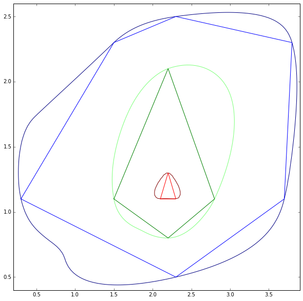
I don't see this as a 2D curve fitting exercise, but rather a 3D one. By considering the data as 3D we can ensure that the curves never cross one another, and can use information from other contours to improve our estimate for the current one.

The following iPython extract uses cubic interpolation provided by SciPy. Note that the z values I've plotted aren't important, as long as all the contours are equidistant in height.

In [1]: %pylab inline
        pylab.rcParams['figure.figsize'] = (10, 10)
        Populating the interactive namespace from numpy and matplotlib

In [2]: import scipy.interpolate as si

        xs = np.array([0.0, 0.0, 4.5, 4.5,
                       0.3, 1.5, 2.3, 3.8, 3.7, 2.3,
                       1.5, 2.2, 2.8, 2.2,
                       2.1, 2.2, 2.3])
        ys = np.array([0.0, 3.0, 3.0, 0.0,
                       1.1, 2.3, 2.5, 2.3, 1.1, 0.5,
                       1.1, 2.1, 1.1, 0.8,
                       1.1, 1.3, 1.1])
        zs = np.array([0,   0,   0,   0,
                       1,   1,   1,   1,   1,   1,
                       2,   2,   2,   2,
                       3,   3,   3])
        pts = np.array([xs, ys]).transpose()

        # set up a grid for us to resample onto
        nx, ny = (100, 100)
        xrange = np.linspace(np.min(xs[zs!=0])-0.1, np.max(xs[zs!=0])+0.1, nx)
        yrange = np.linspace(np.min(ys[zs!=0])-0.1, np.max(ys[zs!=0])+0.1, ny)
        xv, yv = np.meshgrid(xrange, yrange)
        ptv = np.array([xv, yv]).transpose()

        # interpolate over the grid
        out = si.griddata(pts, zs, ptv, method='cubic').transpose()

        def close(vals):
            return np.concatenate((vals, [vals[0]]))

        # plot the results
        levels = [1, 2, 3]
        plt.plot(close(xs[zs==1]), close(ys[zs==1]))
        plt.plot(close(xs[zs==2]), close(ys[zs==2]))
        plt.plot(close(xs[zs==3]), close(ys[zs==3]))
        plt.contour(xrange, yrange, out, levels)
        plt.show()

The results here don't look the best, but with so few control points they are still perfectly valid. Note how the green fitted line is pulled out to follow the wider blue contour.