As I didn't find the existing answers to this problem on StackExchange to be satisfying, I will add my own solution here. This uses geosphere package to calculate distance between two polar (latitude, longitude) coordinates.
For a data frame:
> head(coordinates)
        lat      lng distance
21 51.73832 10.72805     6000
31 51.76656 10.85404     6000
64 51.67559 10.82135     5000
70 51.75592 10.85369     5000
80 51.70379 10.79743     2000
89 51.68976 10.88211     6000
use
n <- nls( distance ~ distm(data.frame(lng, lat), c(lng_solution, lat_solution), fun=distHaversine),
          data = coordinates, start=list( lng_solution=10.9278778, lat_solution=51.6675738 ) )
Substitute the coordinates in the last line with your start-point estimate and make sure the unit of distance equals the unit of the dist-function (this is dependent on whatever dist-function you use, such as distHaversine, distRhumb, distMeeus, etc).
(Note that the geosphere package uses the uncommon convention of writing longitude before latitude.)
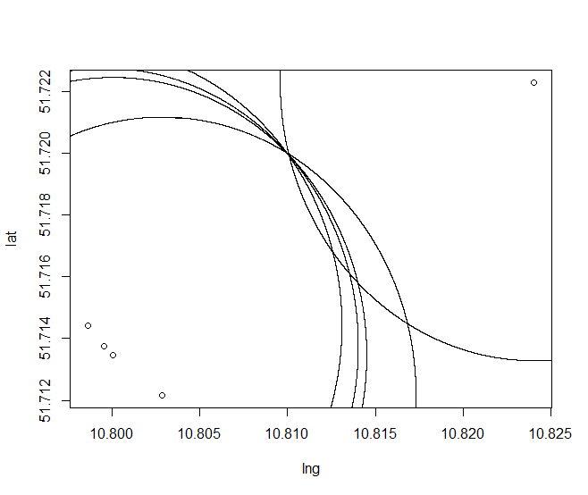
Using the destPoint function of geosphere we can plot the arcs of our measured radii
plot(coordinates[, c("lng", "lat")])
apply(coordinates[, c("lng", "lat", "distance")], 1, function (x) polygon(destPoint(c(x[1], x[2]), b=seq(1, b=1:365, 0.01), d=x[3])))
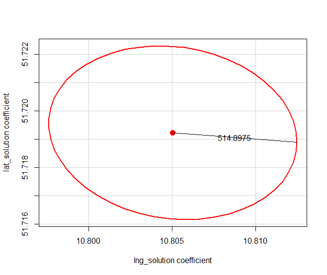
Use the following code to plot the confidence ellipse:
c <- confidenceEllipse(n, levels=0.95)
ellipse_line <- c[1, ]
ellipse_line <- rbind(ellipse_line, coef(n))
lines(ellipse_line)
text(x = mean(ellipse_line[, 1]), y = mean(ellipse_line[, 2]),
     labels=format(distm(ellipse_line[1,], ellipse_line[2,]), nsmall=1))


