added 4 characters in body
Source Link
Stefan
  • 4.5k
  • 1
  • 33
  • 66

The heat map approach:

The approach is more time consuming, due to the calculating time of the processing steps. It could be seen as an idea maybe to get closer to a more general solution.

Test Data:

  • QGIS 2.18.16, GRASS GIS 7
  • 4 GPS Tracks
  • within a grid of 1x1km

I.)

Create points along your GPS Tracks with the QGIS Plugin Locate Points Along Lines (https://plugins.qgis.org/plugins/LocatePoints/). For the heat map approach I've used an interval of 2m.

II.)

Create a heat map with the QGIS heat map plugin. I've used a radius of 40m. I increase the radius until there are no holes in the output raster. You have to try this with different radius values.

enter image description here

III.)

EDITED There is no need to hold the exact heat map raster value.

Now I want to thin out the raster to the "white" areas, where the most points are concentrated. Therefor I recalculate the output raster. The min/max values of the output raster is 0 and 89.7935. I only use values above 44. Therefor I used a "rule of thumb". Round down the max value and divide it by two. Round down this value another time. 89/2 = 44,5 --> 44. I've used the OSGeo4W Shell: gdal_calc -A heatmap.tif --calc="(A>=44)*A"calc="A>=44" --NoDataValue=0 --outfile=heatmap_44_NoData.tif.

enter image description here

IV.)

EDITED

a) Polygonize the recalculated heat map with Raster > Conversion > Polygonize ...

b) Dissolve the output data with Vector > Geoprocessing Tools > Dissolve

c) Simplify the polygon Vector > Geometry Tools > Simplify geometries. I've used a tolerance of 2. A simpler polygon reduces the processing time for the skeletons.

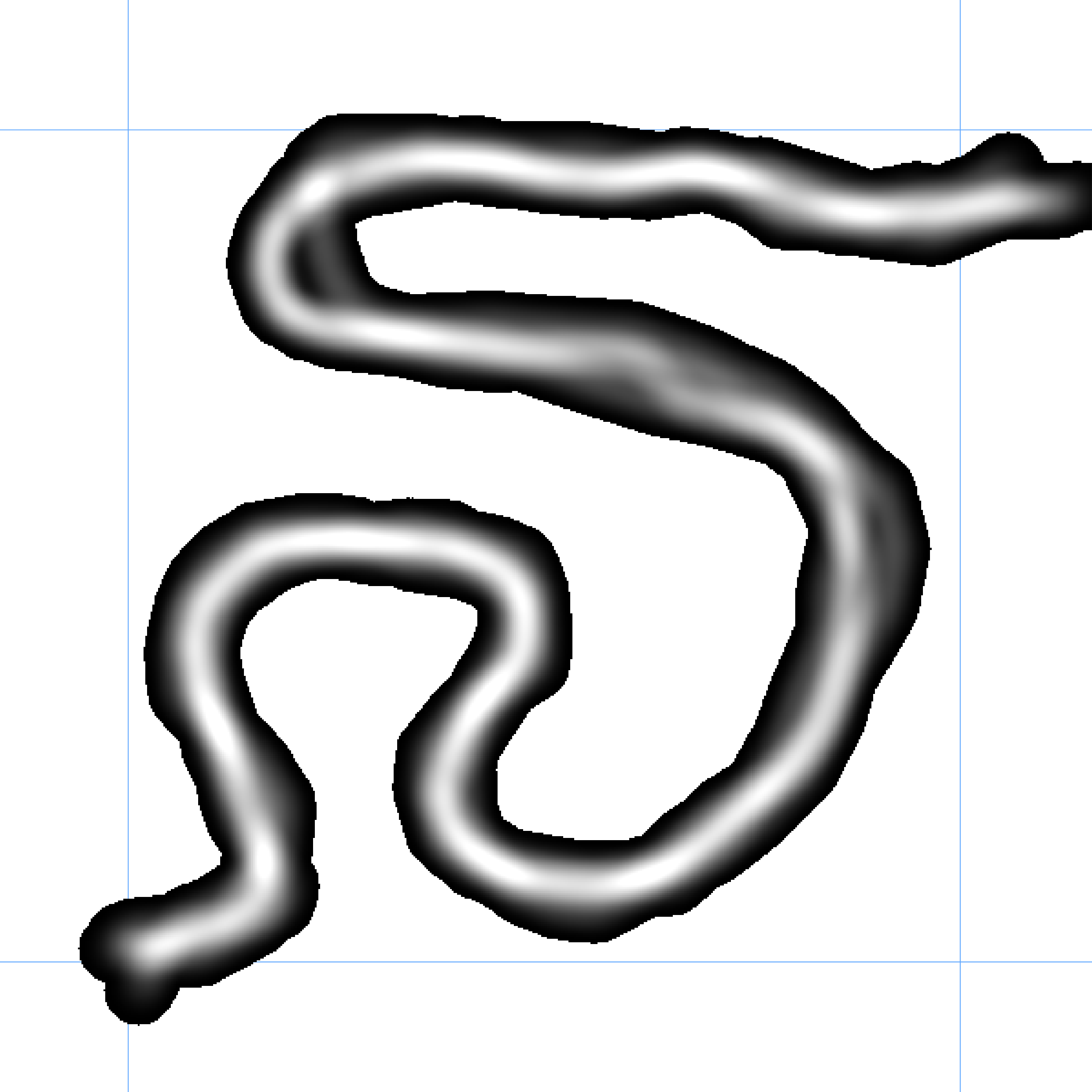
dc) Calculate skeletons: search for skeleton in the Processing Toolbox. Use v.voronoi.skeleton tool from the GRASS GIS 7 commands.

enter image description here

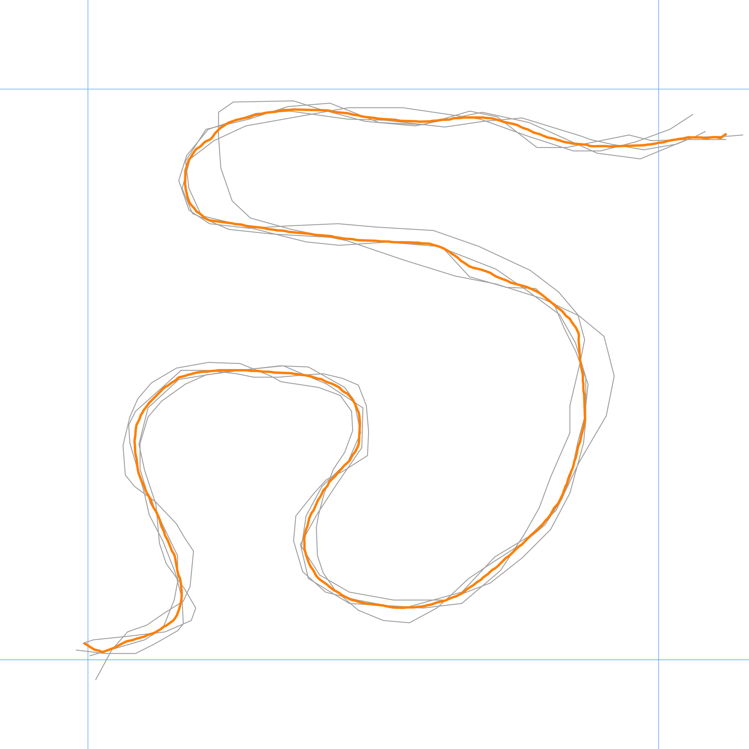
You can see that the resulting line represents more the most probable position of the trail than in my first answer. Especially for the bend in the North the mean line follows the three tracks which are more close to each other. The same for the bend in the East.

Advantages of the approach:

  • reasonable good results exclusively using QGIS

Disadvantages:

  • processing time for big data sets
  • you have to try parameters a priori (radius of heatmap, min/max values )
  • hard to automate the processing steps
  • not tested for narrow bends/curves and for tracks which really step out of the line

If someone can optimize the processing steps, your welcome!

The heat map approach:

The approach is more time consuming, due to the calculating time of the processing steps. It could be seen as an idea maybe to get closer to a more general solution.

Test Data:

  • QGIS 2.18.16, GRASS GIS 7
  • 4 GPS Tracks
  • within a grid of 1x1km

I.)

Create points along your GPS Tracks with the QGIS Plugin Locate Points Along Lines (https://plugins.qgis.org/plugins/LocatePoints/). For the heat map approach I've used an interval of 2m.

II.)

Create a heat map with the QGIS heat map plugin. I've used a radius of 40m. I increase the radius until there are no holes in the output raster. You have to try this with different radius values.

enter image description here

III.)

Now I want to thin out the raster to the "white" areas, where the most points are concentrated. Therefor I recalculate the output raster. The min/max values of the output raster is 0 and 89.7935. I only use values above 44. Therefor I used a "rule of thumb". Round down the max value and divide it by two. Round down this value another time. 89/2 = 44,5 --> 44. I've used the OSGeo4W Shell: gdal_calc -A heatmap.tif --calc="(A>=44)*A" --NoDataValue=0 --outfile=heatmap_44_NoData.tif.

enter image description here

IV.)

a) Polygonize the recalculated heat map with Raster > Conversion > Polygonize ...

b) Dissolve the output data with Vector > Geoprocessing Tools > Dissolve

c) Simplify the polygon Vector > Geometry Tools > Simplify geometries. I've used a tolerance of 2. A simpler polygon reduces the processing time for the skeletons.

d) Calculate skeletons: search for skeleton in the Processing Toolbox. Use v.voronoi.skeleton tool from the GRASS GIS 7 commands.

enter image description here

You can see that the resulting line represents more the most probable position of the trail than in my first answer. Especially for the bend in the North the mean line follows the three tracks which are more close to each other. The same for the bend in the East.

Advantages of the approach:

  • reasonable good results exclusively using QGIS

Disadvantages:

  • processing time for big data sets
  • you have to try parameters a priori (radius of heatmap, min/max values )
  • hard to automate the processing steps
  • not tested for narrow bends/curves and for tracks which really step out of the line

If someone can optimize the processing steps, your welcome!
The heat map approach:

The approach is more time consuming, due to the calculating time of the processing steps. It could be seen as an idea maybe to get closer to a more general solution.

Test Data:

  • QGIS 2.18.16, GRASS GIS 7
  • 4 GPS Tracks
  • within a grid of 1x1km

I.)

Create points along your GPS Tracks with the QGIS Plugin Locate Points Along Lines (https://plugins.qgis.org/plugins/LocatePoints/). For the heat map approach I've used an interval of 2m.

II.)

Create a heat map with the QGIS heat map plugin. I've used a radius of 40m. I increase the radius until there are no holes in the output raster. You have to try this with different radius values.

enter image description here

III.)

EDITED There is no need to hold the exact heat map raster value.

Now I want to thin out the raster to the "white" areas, where the most points are concentrated. Therefor I recalculate the output raster. The min/max values of the output raster is 0 and 89.7935. I only use values above 44. Therefor I used a "rule of thumb". Round down the max value and divide it by two. Round down this value another time. 89/2 = 44,5 --> 44. I've used the OSGeo4W Shell: gdal_calc -A heatmap.tif --calc="A>=44" --NoDataValue=0 --outfile=heatmap_44_NoData.tif.

enter image description here

IV.)

EDITED

a) Polygonize the recalculated heat map with Raster > Conversion > Polygonize ...

b) Simplify the polygon Vector > Geometry Tools > Simplify geometries. I've used a tolerance of 2. A simpler polygon reduces the processing time for the skeletons.

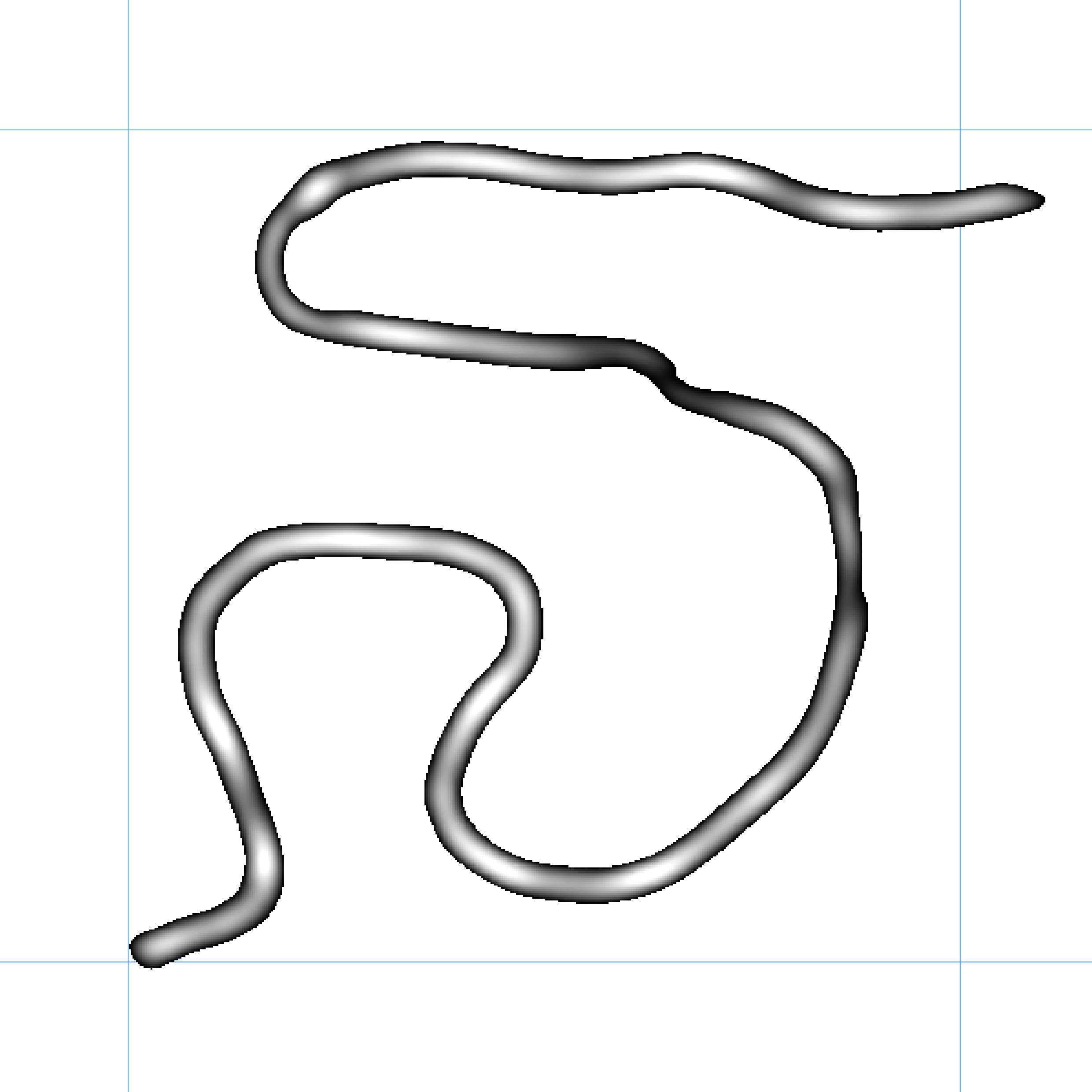
c) Calculate skeletons: search for skeleton in the Processing Toolbox. Use v.voronoi.skeleton tool from the GRASS GIS 7 commands.

enter image description here

You can see that the resulting line represents more the most probable position of the trail than in my first answer. Especially for the bend in the North the mean line follows the three tracks which are more close to each other. The same for the bend in the East.

Advantages of the approach:

  • reasonable good results exclusively using QGIS

Disadvantages:

  • processing time for big data sets
  • you have to try parameters a priori (radius of heatmap, min/max values )
  • hard to automate the processing steps
  • not tested for narrow bends/curves and for tracks which really step out of the line

If someone can optimize the processing steps, your welcome!
Source Link
Stefan
  • 4.5k
  • 1
  • 33
  • 66

The heat map approach:

The approach is more time consuming, due to the calculating time of the processing steps. It could be seen as an idea maybe to get closer to a more general solution.

Test Data:

  • QGIS 2.18.16, GRASS GIS 7
  • 4 GPS Tracks
  • within a grid of 1x1km

I.)

Create points along your GPS Tracks with the QGIS Plugin Locate Points Along Lines (https://plugins.qgis.org/plugins/LocatePoints/). For the heat map approach I've used an interval of 2m.

II.)

Create a heat map with the QGIS heat map plugin. I've used a radius of 40m. I increase the radius until there are no holes in the output raster. You have to try this with different radius values.

enter image description here

III.)

Now I want to thin out the raster to the "white" areas, where the most points are concentrated. Therefor I recalculate the output raster. The min/max values of the output raster is 0 and 89.7935. I only use values above 44. Therefor I used a "rule of thumb". Round down the max value and divide it by two. Round down this value another time. 89/2 = 44,5 --> 44. I've used the OSGeo4W Shell: gdal_calc -A heatmap.tif --calc="(A>=44)*A" --NoDataValue=0 --outfile=heatmap_44_NoData.tif.

enter image description here

IV.)

a) Polygonize the recalculated heat map with Raster > Conversion > Polygonize ...

b) Dissolve the output data with Vector > Geoprocessing Tools > Dissolve

c) Simplify the polygon Vector > Geometry Tools > Simplify geometries. I've used a tolerance of 2. A simpler polygon reduces the processing time for the skeletons.

d) Calculate skeletons: search for skeleton in the Processing Toolbox. Use v.voronoi.skeleton tool from the GRASS GIS 7 commands.

enter image description here

You can see that the resulting line represents more the most probable position of the trail than in my first answer. Especially for the bend in the North the mean line follows the three tracks which are more close to each other. The same for the bend in the East.

Advantages of the approach:

  • reasonable good results exclusively using QGIS

Disadvantages:

  • processing time for big data sets
  • you have to try parameters a priori (radius of heatmap, min/max values )
  • hard to automate the processing steps
  • not tested for narrow bends/curves and for tracks which really step out of the line

If someone can optimize the processing steps, your welcome!