Return to Answer

added a more efficient way to code it

Source Link

edited May 15, 2018 at 14:14

dof1985

3.1k
20
32

library(magrittr)
library(ggplot2)
library(sf)

tt <- read_sf(path, "USA_adm1")

# subset some states to make it plot faster
tt1 <- tt[tt$NAME_1 %in% c("South Dakota", "Wyoming",  
                       "Nebraska", "Iowa"), ]

EDIT - I add another version for this operation, inspired by a very important comment made by spacedman. This would save some computing time, in particular form datasets with multiple points/polygons or complex geometries.

pnts <- data.frame(
"x" = c(-105.08798, -99.61295, -96.22951, 
        -92.35393, -96.59861, -101.45846, -106.87197),
"y" = c(43.27392, 43.48426, 43.05443, 43.04529, 
        43.14589, 42.80751, 44.22843))

# create a points collection
pnts_sf <- do.call("st_sfc",c(lapply(1:nrow(pnts), 
function(i) {st_point(as.numeric(pnts[i, ]))}), list("crs" = 4326))) 

pnts_trans <- st_transform(pnts_sf, 2163) # apply transformation to pnts sf
tt1_trans <- st_transform(tt1, 2163)      # apply transformation to polygons sf

# intersect and extract state name
pnts$region <- apply(st_intersects(tt1_trans, pnts_trans, sparse = FALSE), 2, 
               function(col) { 
                  tt1_trans[which(col), ]$NAME_1
               })

tt <- read_sf(path, "USA_adm1")

# subset some states to make it plot faster
tt1 <- tt[tt$NAME_1 %in% c("South Dakota", "Wyoming",  
                       "Nebraska", "Iowa"), ]

library(magrittr)
library(ggplot2)
library(sf)

tt <- read_sf(path, "USA_adm1")

# subset some states to make it plot faster
tt1 <- tt[tt$NAME_1 %in% c("South Dakota", "Wyoming",  
                       "Nebraska", "Iowa"), ]

pnts <- data.frame(
"x" = c(-105.08798, -99.61295, -96.22951, 
        -92.35393, -96.59861, -101.45846, -106.87197),
"y" = c(43.27392, 43.48426, 43.05443, 43.04529, 
        43.14589, 42.80751, 44.22843))

# create a points collection
pnts_sf <- do.call("st_sfc",c(lapply(1:nrow(pnts), 
function(i) {st_point(as.numeric(pnts[i, ]))}), list("crs" = 4326))) 

pnts_trans <- st_transform(pnts_sf, 2163) # apply transformation to pnts sf
tt1_trans <- st_transform(tt1, 2163)      # apply transformation to polygons sf

# intersect and extract state name
pnts$region <- apply(st_intersects(tt1_trans, pnts_trans, sparse = FALSE), 2, 
               function(col) { 
                  tt1_trans[which(col), ]$NAME_1
               })

Source Link

created May 14, 2018 at 8:12

dof1985

3.1k
20
32

What you are looking can be done using sf::st_intersects() as commented. I provide a full working example using USA states.

tt <- read_sf(path, "USA_adm1")

# subset some states to make it plot faster
tt1 <- tt[tt$NAME_1 %in% c("South Dakota", "Wyoming",  
                       "Nebraska", "Iowa"), ]

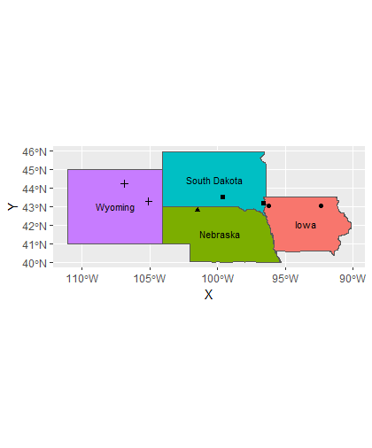
I've added labels over the polygons centroids and now the plot looks like that.

Now for the actual work. Assume a data.frame of lat-lon values.

pnts
           x        y
1 -105.08798 43.27392
2  -99.61295 43.48426
3  -96.22951 43.05443
4  -92.35393 43.04529
5  -96.59861 43.14589
6 -101.45847 42.80751
7 -106.87197 44.22843

pnts$region <- apply(pnts, 1, function(row) {  
   # transformation to palnar is required, since sf library assumes planar projection 
   tt1_pl <- st_transform(tt1, 2163)   
   coords <- as.data.frame(matrix(row, nrow = 1, 
     dimnames = list("", c("x", "y"))))   
   pnt_sf <- st_transform(st_sfc(st_point(row),crs = 4326), 2163)
   # st_intersects with sparse = FALSE returns a logical matrix
   # with rows corresponds to argument 1 (points) and 
   # columns to argument 2 (polygons)

   tt1_pl[which(st_intersects(pnt_sf, tt1_pl, sparse = FALSE)), ]$NAME_1 
})

The results are shown below

           x        y       region
1 -105.08798 43.27392      Wyoming
2  -99.61295 43.48426 South Dakota
3  -96.22951 43.05443         Iowa
4  -92.35393 43.04529         Iowa
5  -96.59861 43.14589 South Dakota
6 -101.45847 42.80751     Nebraska
7 -106.87197 44.22843      Wyoming

and in a plot