A common misconception is that kriging estimates may be simply exponentiated to recover the field values.

Sebastien Rochette's fantastic answer on this thread explains that since the prediction of log(y) is based on a Gaussian distribution, the back-transformation following Laurent (1963) should look like this:

There is a large literature on this topic, and in many cases an additional correction factor is needed because the expected value of back-transformed lognormal kriging estimates is biased, in other words not equal to the sample mean. One method is to multiply the above equation by a correction factor, which is the ratio of the sample mean to the back-transformed means.

Here is a fantastic paper dealing with the issue of back-transforming kriging estimates. It draws on the seminal work on (Journel, 1978).

And here is a fully reproducible example in R:

# load required packages, and download missing ones
if (!require("pacman")) install.packages("pacman")
pacman::p_load(sp, raster, gstat, ggplot2, magrittr)

data(meuse) # load the meuse data set

# convert meuse into a spatial object
# first, prepare the 3 components: coordinates, data, and proj4string
coords <- meuse[ , c("x", "y")]   # coordinates
data   <- meuse[ , 3:14]          # data
crs    <- CRS("+init=epsg:28992") # proj4string of coords

# make the spatial points data frame object
d <- SpatialPointsDataFrame(coords      = coords,
                            data        = data, 
                            proj4string = crs)

r <- raster(d)                       # create raster to interpolate over
res(r) <- 100                        # raster resolution (100 meters)
g <- as(r, "SpatialGrid")            # convert raster to spatial grid object


d$zinc <- log(d$zinc)                # log transform field values
  
gs <- gstat(formula = zinc ~ 1,      # spatial data, so fitting xy as idp vars
            locations = d)           # spatial object
  
v <- variogram(gs,                   # gstat object
               width = 25)           # lag distance
  
# plot the variogram
# plot(v)                              

fve <- fit.variogram(v,              # takes `gstatVariogram` object
                     vgm(0.6,        # partial sill: semivariance at the range
                         "Exp",      # linear model type
                         1000,       # range: distance where model first flattens out
                         0.01))      # nugget
  
# plot variogram and fit
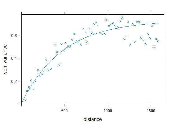
plot(v, fve)

# ordinary kriging 
kp <- krige(zinc ~ 1, d, g, model = fve)
  
# backtransformed
bt <- exp( kp@data$var1.pred + (kp@data$var1.var / 2) )
  
# means of backtransformed values and the sampled values
mu_bt <- mean(bt)
mu_original <- mean(exp(d$zinc))
  
# these means differ...  
> mu_bt
[1] 673.0071
> mu_original
[1] 469.7161

# ...thus make another correction to remove kriging bias in sample mean
btt <- bt * (mu_original/mu_bt)             # correct backtransfomed vals
kp@data$var1.pred <- btt                    # overwrite w/ correct vals 
names(kp) <- c("Prediction", "variance")
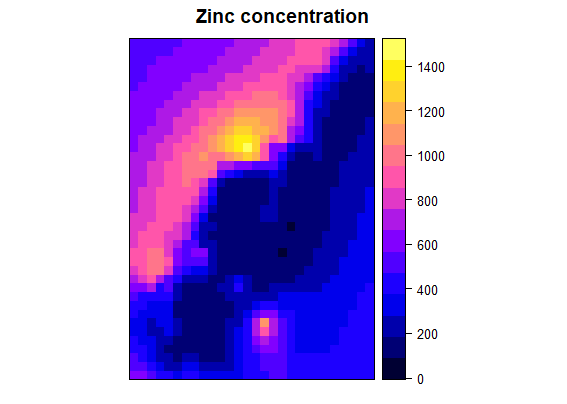
spplot(kp, "Prediction", main = "Zinc concentration")

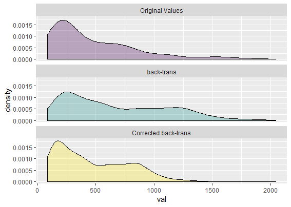
# we can view the motivation for this transformation by comparing the 
# original zinc values to the kirging estimates generated by the
# backtransformation, and the corrected backtransformation
rbind.data.frame(
  data.frame(val = exp(d$zinc), class = "Original Values"), 
  data.frame(val = bt,          class = "Back-trans"), 
  data.frame(val = btt,         class = "Corrected Back-trans")
) %>% 
  ggplot(aes(val)) + 
  geom_density(aes(fill=class), alpha = 0.3) +
  facet_wrap(~class, ncol=1) +
  guides(fill = FALSE)

Summary

It's clear that the density distribution of the corrected backtransform aligns with the sample density distribution, indicating less bias compared to the simple backtransformation without the correction coefficient.