Reference added
Source Link
Taras
  • 34k
  • 4
  • 73
  • 148

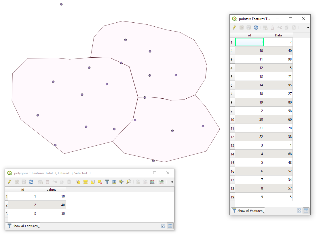
Let's assume there are two layers "points" and "polygons" with its corresponding attribute tables accordingly, see image below.

example

I will try to explain the how-to of both algorithms by means of Spatial SQL using a most-common intersects predicate.

Join attributes by location

This algorithm takes an input vector layer and creates a new vector layer that is an extended version of the input one, with additional attributes in its attribute table.

The additional attributes and their values are taken from a second vector layer. A spatial criteria is applied to select the values from the second layer that are added to each feature from the first layer in the resulting one.

"Join attributes by location" (one-to-many) can be interpreted as

SELECT p.*, poi.*
FROM "polygons" AS p
JOIN "points" AS poi ON st_intersects(p.geometry, poi.geometry)

So, in the result you will see polygons as many times as the intersection between point and polygon exists.

result_1

Join attributes by location (summary)

This algorithm takes an input vector layer and creates a new vector layer that is an extended version of the input one, with additional attributes in its attribute table.

The additional attributes and their values are taken from a second vector layer. A spatial criteria is applied to select the values from the second layer that are added to each feature from the first layer in the resulting one.

The algorithm calculates a statistical summary for the values from matching features in the second layer (e.g. maximum value, mean value, etc).

"Join attributes by location (summary)" can be interpreted as

SELECT p.*, SUM(poi.Data)
FROM "polygons" AS p
JOIN "points" AS poi ON st_intersects(p.geometry, poi.geometry)
GROUP BY p.id

So, in the result you will see limited amount of polygons based on the intersection between points and polygons because the SUM()-function was applied which groups values from points per polygon.

result_2


References:

Let's assume there are two layers "points" and "polygons" with its corresponding attribute tables accordingly, see image below.

example

I will try to explain the how-to of both algorithms by means of Spatial SQL using a most-common intersects predicate.

Join attributes by location

This algorithm takes an input vector layer and creates a new vector layer that is an extended version of the input one, with additional attributes in its attribute table.

The additional attributes and their values are taken from a second vector layer. A spatial criteria is applied to select the values from the second layer that are added to each feature from the first layer in the resulting one.

"Join attributes by location" (one-to-many) can be interpreted as

SELECT p.*, poi.*
FROM "polygons" AS p
JOIN "points" AS poi ON st_intersects(p.geometry, poi.geometry)

So, in the result you will see polygons as many times as the intersection between point and polygon exists.

result_1

Join attributes by location (summary)

This algorithm takes an input vector layer and creates a new vector layer that is an extended version of the input one, with additional attributes in its attribute table.

The additional attributes and their values are taken from a second vector layer. A spatial criteria is applied to select the values from the second layer that are added to each feature from the first layer in the resulting one.

The algorithm calculates a statistical summary for the values from matching features in the second layer (e.g. maximum value, mean value, etc).

"Join attributes by location (summary)" can be interpreted as

SELECT p.*, SUM(poi.Data)
FROM "polygons" AS p
JOIN "points" AS poi ON st_intersects(p.geometry, poi.geometry)
GROUP BY p.id

So, in the result you will see limited amount of polygons based on the intersection between points and polygons because the SUM()-function was applied which groups values from points per polygon.

result_2


References:

Source Link
Taras
  • 34k
  • 4
  • 73
  • 148

Let's assume there are two layers "points" and "polygons" with its corresponding attribute tables accordingly, see image below.

example

I will try to explain the how-to of both algorithms by means of Spatial SQL using a most-common intersects predicate.

Join attributes by location

This algorithm takes an input vector layer and creates a new vector layer that is an extended version of the input one, with additional attributes in its attribute table.

The additional attributes and their values are taken from a second vector layer. A spatial criteria is applied to select the values from the second layer that are added to each feature from the first layer in the resulting one.

"Join attributes by location" (one-to-many) can be interpreted as

SELECT p.*, poi.*
FROM "polygons" AS p
JOIN "points" AS poi ON st_intersects(p.geometry, poi.geometry)

So, in the result you will see polygons as many times as the intersection between point and polygon exists.

result_1

Join attributes by location (summary)

This algorithm takes an input vector layer and creates a new vector layer that is an extended version of the input one, with additional attributes in its attribute table.

The additional attributes and their values are taken from a second vector layer. A spatial criteria is applied to select the values from the second layer that are added to each feature from the first layer in the resulting one.

The algorithm calculates a statistical summary for the values from matching features in the second layer (e.g. maximum value, mean value, etc).

"Join attributes by location (summary)" can be interpreted as

SELECT p.*, SUM(poi.Data)
FROM "polygons" AS p
JOIN "points" AS poi ON st_intersects(p.geometry, poi.geometry)
GROUP BY p.id

So, in the result you will see limited amount of polygons based on the intersection between points and polygons because the SUM()-function was applied which groups values from points per polygon.

result_2