ArcGIS quantile classification method results in unequal data values in each class

Question

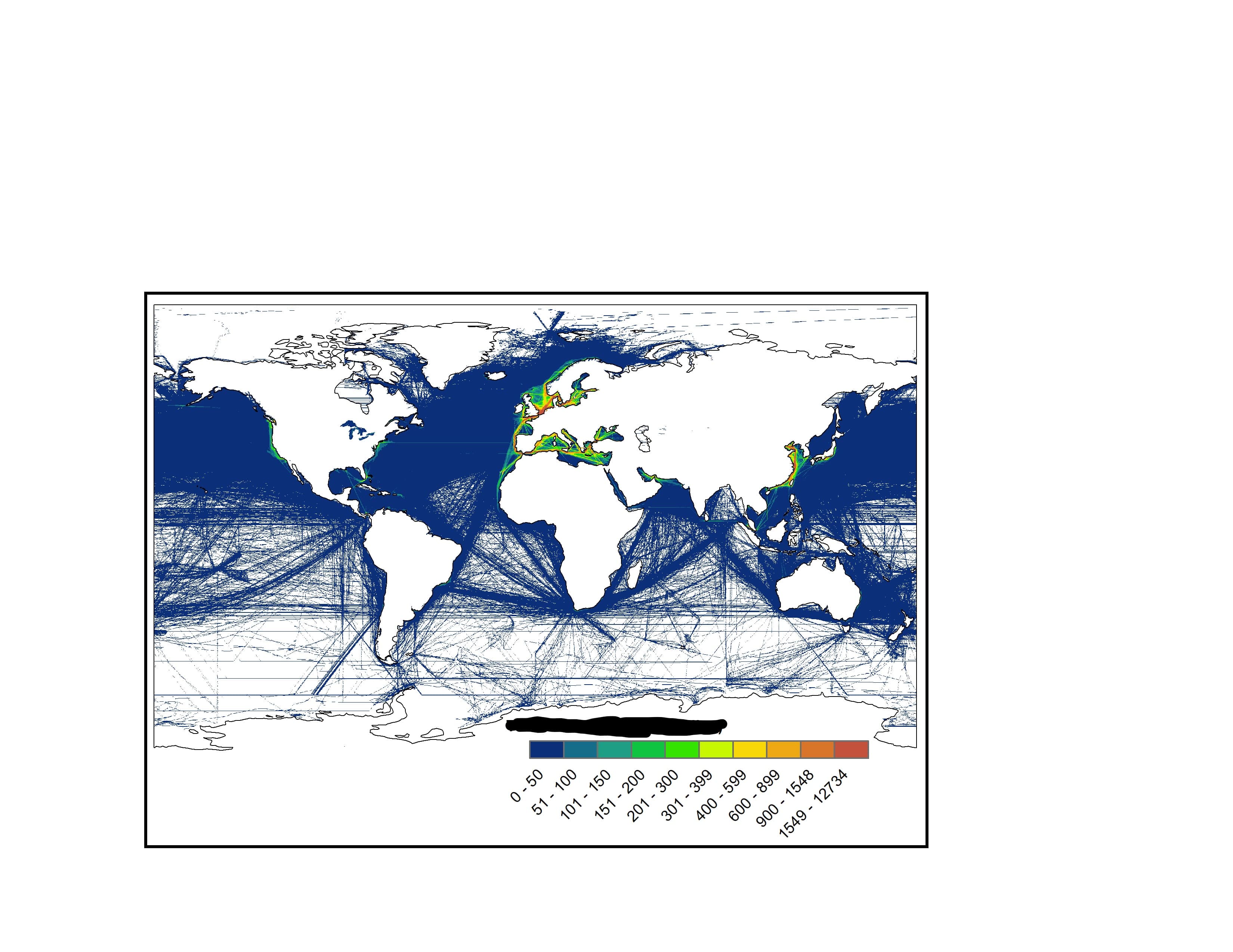
I have a raster dataset which I visualized in ArcMap 10.6.1. I used the quantile data classification method to assign colours to the data values. ESRI's documentation says the following about quantiles: "Quantile assigns the same number of data values to each class". Thus, I would expect a raster map that looks something like this. However, I end up with the map below.

Does anyone have an explanation for the unexpected outcome of the quantile classification? Could it have something to do with the distribution of the values? All values in the open ocean are very low (0-50), while values near coastlines can be very high (up to 12734). Unfortunately I am not allowed to share the actual data due to confidentiality.

Answer 1

You may be trying to force quantiles with too many bins based on your data. I see 10 quantiles in your legend. For sake of example, let's imagine there are 1 million pixels on the board. Each quantile should then get 100,000 pixels. Your lowest bin has values in the range of 0-50. I don't know your data, but what happens if you have, say 600,000 pixels all with the value of 50? That's already more pixels than will fit into one bin. How does ArcGIS split this collection of pixels into separate bins when they are the same value? If you try symbolizing with 3 quantiles do you get a more reasonable result? I have run into this situation of too many of the same or similar value features using python scripts, and it typically fails to create the number of bins or breakpoints that I've specified. I'm not sure what kind of behavior to expect when performing the symbology manually in ArcMap. Check that your data has enough spread to support this number of bins.

Answer 2

Quantile classification or symbology will group the same number of entries into each category. In a vector symbology context this would mean if you had 1000 items and 10 categories, each category would have 100 items in it. I would assume in a raster context it would be similar, with the same number of pixels in each category. Looking at your legend it appears that your data has a skewed distribution with a right tail, so the higher values are more spread out than the lower values. This would mean the thresholds between categories would be closer together at lower values.

Looking at your map (which appears to be vector data instead of raster data?) I wonder if the reason why there appear to be so many more low value shipping routes is that the long distance routes take up more space. In other words, ten routes that each cover 1000 miles which show up more easily on this map than ten routes that each cover only 5 miles. If you zoomed into one of the coastline areas with high value routes would you find a greater density of short distance routes?