How to crop an ASCII file?

Question

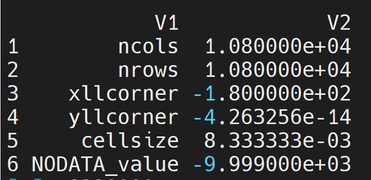
I have data downloaded from https://sedac.ciesin.columbia.edu/data/set/gpw-v4-population-count-rev11. It is in an ASCII file, and I want to plot the map and the populations of just California. What is the easiest way to locate the grid cells in California?

Answer 1

As said in my answer to your other (deleted) question,

This is ESRI ascii grid file for rasters. You can convert the text-based ascii grid files to other formats using ArcGIS tools under ArcToolbox\Conversion Tools\ From Raster and To Raster categories.

And then, you can plot/crop the image file however you like.

Answer 2

So the full workflow would be:

1. Get your raster
2. Get a shapefile of California
3. Ensure the shapefile is on the same CRS than your raster
4. Crop the raster using your shapefile.

With the raster package:

library(raster)
#> Warning: package 'raster' was built under R version 4.1.3
#> Loading required package: sp
#> Warning: package 'sp' was built under R version 4.1.3

init_raster <- raster()

init_raster
#> class      : RasterLayer 
#> dimensions : 180, 360, 64800  (nrow, ncol, ncell)
#> resolution : 1, 1  (x, y)
#> extent     : -180, 180, -90, 90  (xmin, xmax, ymin, ymax)
#> crs        : +proj=longlat +datum=WGS84 +no_defs

# Get California
library(nominatimlite)
california <- geo_lite_sf("California, USA", points_only = FALSE)
california
#> Simple feature collection with 1 feature and 2 fields
#> Geometry type: MULTIPOLYGON
#> Dimension:     XY
#> Bounding box:  xmin: -124.482 ymin: 32.52952 xmax: -114.1308 ymax: 42.0095
#> Geodetic CRS:  WGS 84
#>             query                   address                       geometry
#> 1 California, USA California, United States MULTIPOLYGON (((-124.482 40...

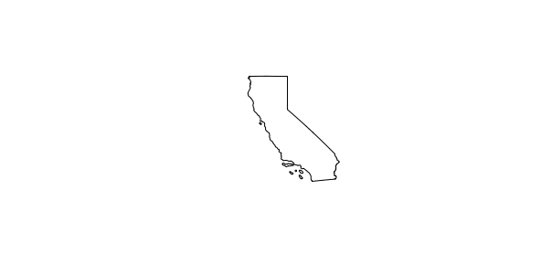
plot(sf::st_geometry(california))

# Crop

library(sf)
# Ensure the same sf
california <- st_transform(california, crs=crs(init_raster))

raster_california <- crop(init_raster, california )

raster_california
#> class      : RasterLayer 
#> dimensions : 9, 10, 90  (nrow, ncol, ncell)
#> resolution : 1, 1  (x, y)
#> extent     : -124, -114, 33, 42  (xmin, xmax, ymin, ymax)
#> crs        : +proj=longlat +datum=WGS84 +no_defs

^{Created on 2022-06-24 by the reprex package (v2.0.1)}

Note the extent of raster_california and the Bounding box of california