3

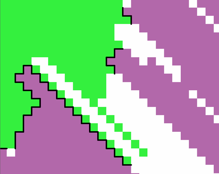
Is there a way in R to create lines (black lines in the figure below) along the edge between two raster cells that have different values ?

enter image description here

Update

I'm trying the functions clump() and rasterToPolygons() as in the post [https://stackoverflow.com/questions/28859181/how-to-get-contour-lines-around-the-grids-in-r-raster].

First, I reclassified my raster "r" to have cells with two different values:

new.values <- cbind(c(0, 1, 2, 3, 4, 5, 6, 7, 8), c(NA, NA, 1, NA, 2, NA, NA, NA, NA))
new.r <- reclassify(r, rcl=new.values)

Then, I used the functions rasterToPolygons and clump:

test.edge <- rasterToPolygons(clump(new.r), dissolve=TRUE)
plot(test.edge, add=TRUE)

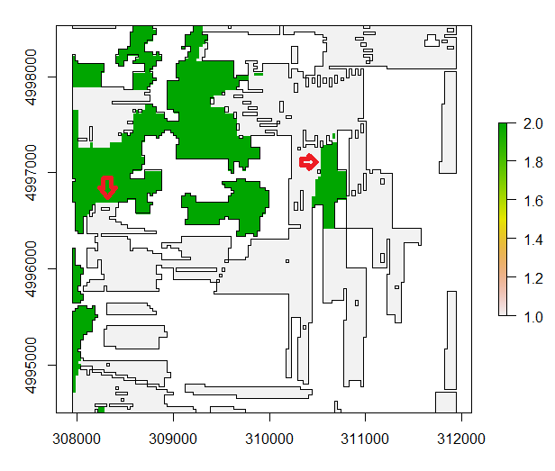
And I obtained:

enter image description here

How can I extract the edges that have not contour lines (for example, edges near red arrows) because they are located between two different values?

1

2 Answers 2

3

I think it is not wise to mix the clump(..) functionality from igraph with the dissolve=TRUE parameter from the rasterToPolygon routine. They both do something with to aggregate the fields together but in a different way. At least we want to do 3 things:

  1. read or desing a raster
  2. select raster area where the contour goes around
  3. define how the contour is shaped (rectangular,linear or smooth) and define which areas belong together.

In the clump code raster, the type of raster and the definition of NA seems to be important to steer clumping the process. I made some test but with bad results. I followed your sketch and here is a little analysis how to get things work:

# Load packages
require('raster')
require('rgeos')

# Clean up everything
rm(list=ls())

# Set a defined random seed
set.seed(2)

# Create a float raster with values
# the interval [0,2] float
rs <- raster(nrow=10, ncol=10)

# Scale the random numbers from interval [0,1) to
# to [0,2.2) and shift the interval to [-0.1,2.1)
rs[] <- runif(ncell(rs)) * 2.2 - 0.1

# Cut off the raster values to [0,2]
# Everything smaller then 0 is zero
values(rs)[values(rs) < 0.0] <- 0.0

# Everything larger then 2 is two
values(rs)[values(rs) > 2.0] <- 2.0

Is the raster field well constructed?

# Construction is OK?
> quantile(values(rs))
       0%       25%       50%       75%      100% 
0.0000000 0.3928834 0.8733250 1.6027794 2.0000000 

Here is the function prototype that selects the field in the interval [1,2).

# Function of the contour ID
inOne <- function(x) { x>=1 & x<2 }

> inOne(0) 
[1] FALSE

> inOne(1) 
[1] TRUE

> inOne(2)
[1] FALSE

The contour cannot be dissolved (clump) because of the float number nature of the raster field is distinct in the ID process (dissolve-=TRUE).

# Contour of the float desing
# x := [1,2)
ct <- rasterToPolygons(rs, 
         fun=inOne , 
         dissolve=TRUE) 
plot(rs)
plot(ct, add=TRUE)

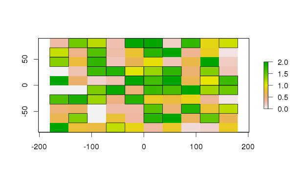
You see the right contour groups, but polygons are not joint.

Float design

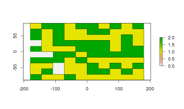
So if we have a unique ID of each cell as Integer, the dissolve process should work.

# Apply integer operation (ceiling, floor, round)
# to the float number fields 
rs.int <- ceiling(rs)
values(rs.int)
ct.int <- rasterToPolygons(rs.int, 
              fun=inOne , 
              dissolve=TRUE) 
plot(rs.int)
plot(ct.int, add=TRUE)

Integer desing

Conclusion: I think (do know not exactly) what behind the clump stuff works a raster based region growing routine. The process dissolve=TRUE in the rasterToPolygon (based on rgeos CRAN) seems to follow a vector approach. So I've to read the manuals of igraph and rgeos carfully.

REM: The selection of contours (float vs. int) differs, because of the nature of (ceiling, floor and round).

4
  • Thank you very much huckfinn for your help. I tested the code but I obtained contour lines around all polygons with cell values that are equal to 1. Is it possible to have the edge between cells with only values that are equal to 1 (yellow) and 2 (green) ? In the second image of your answer, there is edges between cells with values that are equal 1 (yelllow) and 0 (white). I found the function extractedge in the software "GME" [spatialecology.com/gme/extractedge.htm]. The function works very well but I would prefer to use only R. Commented Feb 14, 2016 at 0:09
  • Oh, I think thats the part you have to investigate between the selection function inOne <- function(x) { x>=X & x<Y } and the discretization type rs.int <- ceiling(rs) (floor, round ..also possible ) and a step wise selection (layer 1 is inOn() ..layer 2 is inTwo()...) I guess.
    – huckfinn
    Commented Feb 14, 2016 at 2:07
  • Sorry, I don't know how to do. I still have the contour lines around polygons and not just the edges between two cells like in my first image. Commented Feb 16, 2016 at 4:01
  • Than is the rasterToPolygons not an option to calculate, because polygons enclose areas with one states and the rest out side. You want to separate three states A, B and NA.
    – huckfinn
    Commented Feb 16, 2016 at 11:09
2

I cannot not find some stuff in the raster and rgeos package and wrote a small example that calculates ONLY the segments (egdes in igraph speech) between two layers from scratch, not very fast. To build lines (topologies) from this point is not a straight forward to handle task. One point can join four segments, if you have a chess board pattern for example. If you connect all segments you will get a line graph not a line string. I think there are better solutions and you could investigate the capabilities of igraph.

Here is the script:

# Load packages
require('raster')

# ----------------------------------------
# Create a test raster with 
# cell transitions 2 -> 1
# some open cells at the border 
# and 0 hole in the center
makeTestRaster <- function() {
  nc <-5; nr <-5;
  rs<-raster(nrow=nr,ncol=nc);
  for (c in 1:nc) {
    for (r in 1:nr) {
      if( r==2 | c==2 | r==4 | c==4 ) {
        rs[r,c]=2;
      } 
      else if (r==3 | c == 3)  {
        rs[r,c]=1;
      }
      else {
        rs[r,c]=0;
      }
    }
  }
  rs[3,3] <-0
  return(rs)
}

# ----------------------------------------------
# Calculate all segments with a <-> b connection
# (without a iteration pattern)
# df - the serialized form
# rs - the raster
# pos - pos in the table
# a - cell sourrounded by 
# b - cell neighbor type
calcSegmentAtPos <- function(df,rs, pos, a, b, DEBUG=FALSE) {
  nc<-ncol(rs) # number of columns 
  nr<-nrow(rs) # number of rows
  pcol<-(pos-1) %%   nc + 1; # raster col
  prow<-(pos-1) %/%  nc + 1; # raster row
  result<-c(); # result vector
  # Position in raster OK?
  if (pcol <  0 | prow <  0 |
      pcol > nc | prow > nr ) {
    return (result);
  } 
  # Call is of type A
  if (rs[prow, pcol] != a) return (result);
  # Cell resolution x and y
  dx <- xres(rs);
  dy <- yres(rs);
  # Test positions and type (horizontal, vertical)
  tcol  <- c(pcol-1, pcol+1, pcol,   pcol);
  trow  <- c(prow,   prow,   prow-1, prow+1);
  ttype <- c(TRUE,   TRUE,   FALSE,  FALSE);
  # Run tests and calc segments 
  for (ix in 1:4) {
      scol <- tcol[ix] # test column 
      srow <- trow[ix] # test row
      vertical <- ttype[ix]; # generation type
      # Test position in raster OK?
      if (scol < 1 | scol > nc | 
          srow < 1 | srow > nr ) {
        next;
      }  
      # Test type a <-> b between cells OK ?
      va = rs[prow,pcol]
      vb = rs[srow,scol]
      if (rs[prow,pcol] == a &
          rs[srow,scol] == b) {
        # Somcontraol messages if wanted
        if (DEBUG) {
          cat("pcol", pcol, "| prow", prow, 
            "| scol", scol, "| srow", srow,
            "| a",va,"| b",vb,"| vert", vertical,
            "\n")
        }

        dta <- df[pos, ] # get the data row
        x <- dta$x;      # center of the cell X
        y <- dta$y;      # center of the cell Y
        # Vertical segment
        if ( vertical ){
          x1 <- x + (scol-pcol) * dx/2
          x2 <- x1
          y1 <- y - dy/2
          y2 <- y + dy/2
        } 
        # Horizontal segment
        else {
          y1 <- y + (prow-srow)  * dy/2
          y2 <- y1;
          x1 <- x - dx/2
          x2 <- x + dx/2
        }
        # push data to the result vector
        result<-c(result,c(pos,x,y,x1,y1,x2,y2))
      } # in frame an state a b
  }  #iterate test positions
  return (result) 
}

# --------------------------------------------
# Calculate the segments of over all
# raster points of rs with the transtition a,b
calcSegments <- function(rs, a, b) {

  # Serialized form of the raster
  # with all coordinates
  df <- as.data.frame(rs,xy=TRUE)
  # Understand cell addressing 
  nall <- ncell(rs);
  # df$col <- seq(0,nall-1) %%  nc +1
  # df$row <- seq(0,nall-1) %/% nc +1
  #Resulting segment buffer
  segs <- c();
  for (pos in 1:nall) {
    v <- calcSegmentAtPos(df, rs, pos, a, b);
    if (length(v)>0) segs <-c(segs,v)
  }
  # Re-arrange the segment vector into a data frame
  len<-length(segs)/7; sq <-(0:(len-1))*7 # Index sequenz
  return(data.frame(id=segs[sq+1],
                    x=segs[sq+2],
                    y=segs[sq+3],
                    x0=segs[sq+4],
                    y0=segs[sq+5],
                    x1=segs[sq+6],
                    y1=segs[sq+7]))
}

rs <- makeTestRaster()

# Calculate the segments
df <- calcSegments(rs, 2, 1)

The result is a segment table could be a start point to use igraph to compose a graph.

> head(df)
  id    x  y   x0  y0   x1 y1
1  2  -72 72  -36  54  -36 90
2  4   72 72   36  54   36 90
3  6 -144 36 -180  18 -108 18
4  8    0 36  -36  54   36 54
5 10  144 36  108  18  180 18
6 12  -72  0 -108 -18 -108 18
  • id - index of the raster cell
  • x - center of the cell x
  • y - center of the cell y
  • x0 - start point edge x
  • y0 - start point edge y
  • x1 - end point edge x
  • y1 - end point edge y

The visualisation of the resulting segments looks like this.

# Plot the raster
plot(rs);

# Draw the segments
segments(df$x0,df$y0,df$x1,df$y1)

# Draw the center points
points(df$x,df$y)
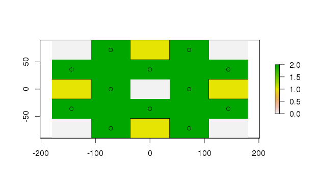
Example

Your Answer

By clicking “Post Your Answer”, you agree to our terms of service and acknowledge you have read our privacy policy.

Not the answer you're looking for? Browse other questions tagged or ask your own question.