10

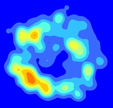
I've created an average kernel density map by running KDEs on points stacked within the same spatial extent. For example, say we have three point shapefiles representing seedlings in three different forest gaps of the same shape and size. I ran a KDE for each point shapefile. The output from the KDE were then stacked based on spatial extent in order to calculate the average in Arc's raster calculator, for example: Float(("KDE1"+"KDE2"+"KDE3")/3). Here is the final product:

enter image description here

Now I'm interested in creating a map depicting the error associated with the averaged KDEs. I hope to use the error map to visually depict how much error is associated with the hotspots (e.g. is the SW hotspot due entirely to the points in one gap?). How should I go about creating a map of the error associated with the averaged KDEs? Would MSE be the most appropriate measure of error in this case?

2
  • 3
    It's very interesting analysis. What do you mean by "standard error"? Some kind of deviation (difference) each density map from "mean" layer? Commented Jan 8, 2013 at 20:01
  • @Landscape Analysis Post edited to adress comments. Yes, I'm thinking that a MSE estimate might be most appropriate in this case. Essentially, showing how each KDE diverges from the average KDE. I'm not sure how to put this all together using ArcGIS and/or scripting though.
    – Aaron
    Commented Jan 8, 2013 at 20:23

1 Answer 1

8

A Caveat

A standard error is a useful way to estimate an uncertainty from sampled data when there is no systematic error in the data. That assumption is of dubious validity in this context, because (a) the KDE maps will locally have definite errors that may persist systematically among the layers and (b) a potentially huge component of uncertainty due to the choice of kernel radius (or "bandwidth") will not be reflected at all in any one given collection of these maps.

Some Choices

Nevertheless, portraying the variability among a collection of related, collocated ("stacked") maps is a great idea--provided you remember the limitations just described. Several measures of local variability would be natural in this setting, including:

  • The range of values, expressed either additively (maximum minus minimum) or multiplicatively (maximum divided by minimum).

  • The variance or standard deviation of values. The multiplicative version of this would be the variance or standard deviation of the logarithms of the values.

  • A robust estimator of dispersion, such as the interquartile range (or the ratio of the third to first quartiles).

In many respects, the multiplicative measures may be more appropriate for densities, because the difference between (say) 100 and 101 trees per acre may be inconsequential whereas the difference between 2 and 1 trees per acre could be relatively important. Both exhibit the same (additive) range of 101 - 100 = 2 - 1 = 1, but their multiplicative ranges of 1.01 and 2.00 differ substantially. (Notice that a multiplicative range always exceeds 1, so that 2.00 is one hundred times further from 1 than 1.01 is.)

Computation

Computing these measures requires some form of local statistics. The cell statistics functionality in Spatial Analyst will compute the variances, ranges, and standard deviations. The local quantiles can be found with rank. Rather than being fussy about which ranks to use, pick convenient ones near the quartiles. To find them, let n be the number of grids in the stack. The median has a rank of (n+1)/2--which might not be a whole number, indicating it should be computed by averaging the n/2 and n/2 + 1 ranks, either of which would approximate the median. To approximate the quartiles, then, round (n+1)/2 down to the nearest whole number, then again add 1 and divide by 2. Let this number be r. Use r and n + 1 - r for the ranks of the quartiles.

As an example, if the stack has n = 6 grids, (n+1)/2 rounded down is 3 and (3+1)/2 = 2 needs no rounding. Use r = 2 and r = 6 + 1 - 2 = 5 for the ranks. In effect, this procedure would return the second lowest (r = 2) and second highest (r = 5) value of the six values at each cell. You could map either their difference or their ratio.
4
  • 2
    I would imagine that the coefficient of variation would be useful in this context. Commented Jan 8, 2013 at 22:24
  • 1
    @jeffrey Thank you, that is a consideration, too. The CV is obtained by dividing the (local) standard deviation grid by the (local) mean grid. I didn't mention it, but for such multiplicative summaries, some care should be taken to mask out areas where the denominator (the mean or minimum, as the case may be) is close to zero: the results may be unreliable there and likely will reflect nothing other than numerical imprecision and tiny inaccuracies in approximating the kernels.
    – whuber
    Commented Jan 8, 2013 at 23:40
  • @whuber, could you elaborate on (a) in your first paragraph? For example, are you referring to errors in data collection techniques that may persist across each forest gap (and therefore systematically manifest themselves in each KDE raster), or errors tied to the implementation of the focal function?
    – MannyG
    Commented Jan 9, 2013 at 1:23
  • @MannyG The former, especially when the sampling points are not sampled randomly or systematically (i.e, on a grid).
    – whuber
    Commented Dec 13, 2023 at 22:26

Your Answer

By clicking “Post Your Answer”, you agree to our terms of service and acknowledge you have read our privacy policy.

Not the answer you're looking for? Browse other questions tagged or ask your own question.