3

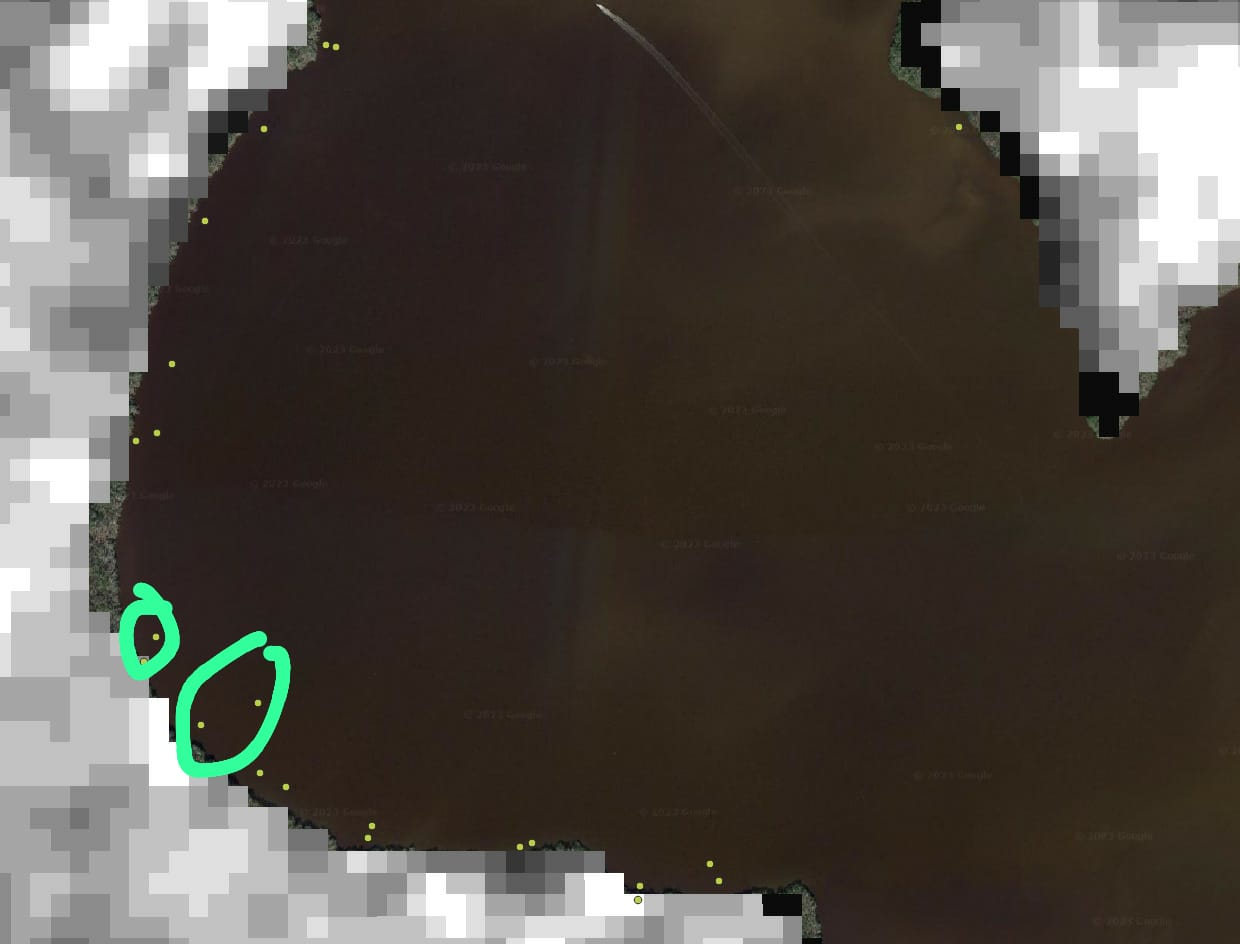
points in lagoon

We have points data which represent places we tied a gillnet (imagine a tennis net underwater) to mangrove roots along the shoreline and subsequently caught (and released) sawfish, a type of shark. All these points SHOULD be against the shore but various inaccuracies mean they aren't. Compounding the issue, the raster data we need (mangrove height from LIDAR) seems to only include pixels where the majority is land, so many near-shore pixels don't have mangrove values.

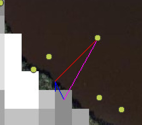
distance

Therefore, I want to attach/join the raster (continuous) values to the points based on nearest distance to mangrove data, i.e. the point above would take the pink line to nearest mangrove point, and get that value.

In R, I used terra::distance, which replaces raster::gridDistance, being much faster. This took 48 hours, but now I have a raster of the distances to the mangrove raster, but obviously don't have the values for the nearest pixel.

While this may still be useful since I need to cutoff any distances above 200m (and so I could use it as a mask), I still can't think how to get the value from the nearest distance mangrove pixel.

Identifying value of closest non-NA pixel is similar but note the comments on the answer - this doesn't seem to apply to continuous data. I've asked Robert Hijmans about adding this capability into terra::distance, but I'm wondering if there's a way to achieve this otherwise.

Do you have any ideas for how to do this using R?

0

2 Answers 2

2

From a GIS perspective, a buffer approach is often what immediately comes to mind. However, in R and general spatial statistical parlance, this is a kNN (nearest neighbor, distance matrix) type problem and can be solved much more efficiently than using a vector topology solution, which can become unwieldy with certain types of large data and intersection operators. For the raster distance analysis, I would recommend using the rasterDistance function in spatialEco as it is basically the same as the distance function available in terra with the exception that I use the Arya & Mount Approximate Near Neighbor (ANN) C++ library for calculating distances, rather than stats::dist, which is orders of magnitude faster.

Here is a solution that uses the ANN C++ library for addressing a kNN type problem. I will note that this is not memory safe so, if you have a very large raster, where coerced points will not fit into RAM, a buffer solution may be more computationally safe, albeit considerably slower. Memory issues are unfortunately generally the case, even with the terra::distance function as, some type of distance function is required necessitating a matrix of coordinates on the x and y side. The dimensionality explodes rather quickly however, the ANN approach has some computational shortcuts that mitigates the issue of nXn matrices representing all of the [x,y] data. One thing that you could do to generally speed up your analysis is to buffer all of your points to the constrained distance and then mask your raster to the resulting buffers. This would notably limit the size of the problem and speed things up. Although, I do not do this in my example.

First, add libraries and create some example data where s = a single value raster [1]; pts = sf POINT object with random sample of n=10; s.pts = sf POINT object of the s raster.

library(terra)
library(sf)
library(RANN)

s <- project(rast(system.file("ex/elev.tif", 
             package = "terra")), "EPSG:5070")
pts <- st_as_sf(spatSample(s, 10, method="random", 
                na.rm=TRUE, as.points=TRUE))
  s <- ifel(s > 350, 1, NA) 
    s.pts <- st_as_sf(as.points(s))
 
plot(st_geometry(pts))
  plot(s, add=TRUE)
    plot(st_geometry(pts), pch=20, cex=2, 
         col="red", add=TRUE)

Here we use the RANN library to derive k nearest neighbors within a specified search radius. The nn.idx object is a matrix of the nearest neighbors row indices, which includes self-realized neighbors (thus, k=2 and not 1) so, you want the second column. If there is no matching neighbor within the search radius then a 0 is returned. This ensures that the resulting matrix matches the dimension of the query. We take this matrix and apply an ifelse statement that turns 0 values to NA’s and can then pipe the resulting vector directly into the original point data. We can also query the raster points to subset to the identified kNN points. Remember that the new column in the original point data will represent the row index of the raster points. Finally, we can create a distance matrix of the kNN observations. Note, I am using outer parentheses to simply print objects.

rad = 1000  # search radius (in projected distance units)
k = 2       # can increase number of neighbors
 
( nn.idx <- RANN::nn2(st_coordinates(s.pts)[,1:2], 
            query = st_coordinates(pts)[,1:2], k = k, 
            searchtype = "radius", radius = rad)$nn.idx )            
( nn <- ifelse(nn.idx[,2] > 0, nn.idx[,2], NA) )
 
pts$nn <- nn 
  
( nn.pts <- na.omit(s.pts[nn,]) )
 
plot(st_geometry(pts), pch=20)
  plot(nn.pts, add=TRUE, pch=20, col="red", cex=2)
 
( d <- st_distance(nn.pts, pts) )

One thing that I will point out is that, if rm.na=FALSE in the terra::as.points function, the row names in the resulting raster points are the same as the cell ID’s, which opens up numerous possibilities in further analysis. We can track this by creating a vector of the original rownames and an index of NA’s. We then drop the NA values in the points and pipe in the original rownames, sans the NA’s, to the new points. The rownames now match the cell ID’s in the raster and can be indexed, using a single bracket, as needed (see below example). I have found this useful in customized functions (eg., custom prediction, Monte Carlo simulations, temporal analysis, …) that takes data.frame type input requiring piping results into an empty raster representing the dimension of the original data.

s <- rast(system.file("ex/elev.tif", package = "terra")
s.pts <- st_as_sf(as.points(s, na.rm=FALSE))
  ridx <- rownames(s.pts)
  na.idx <- which(is.nan(st_drop_geometry(s.pts[,1])))
 
s.pts <- s.pts[-na.idx,]
  rownames(s.pts) <- ridx[-na.idx]
 
# check if rownames match cell ids
e <- extract(s, vect(s.pts), cells=TRUE)
  head(e$cell)
  head(ridx[-na.idx])
 
# index raster and check against extracted values
head(s[as.numeric(ridx[-na.idx])])
head(e)
1

Answers from SCGIS listserv superheroes:

Chris DeRolph

In Arc, I would convert the raster to points, then use the Near tool (or Spatial Join) to get the value of the closest raster point to each green dot. Hope this helps.

Dave Richardson

If you are already creating the mask based on a 200 m. distance cutoff, then you could use Nibble (ArcGIS/ArcPro) to assign the nearest floating point value to the mask, then extract the values to your points from there. It’ll work with floating point values.

Chris Nicholas

in GRASS, to make the mask one can use r.grow, as per: https://grass.osgeo.org/grass82/manuals/r.grow.html

and "grow" out a polygon to cover the area on shore, then use that mask to categorize everything else as "off shore"

Then you can "clump" adjacent offshore pixels into islands, as per: https://grass.osgeo.org/grass82/manuals/r.clump.html

Then you can use GRASS r.distance, as per: https://grass.osgeo.org/grass82/manuals/r.distance.html

to find the shortest distance, or load the polygons into PostGIS, and do something like:

with on_shore as (select * from loaded_polys where category = 'A'),
category_B as (select * from loaded_polys where category = 'B'), 

(
SELECT ST_Distance("table_A".geom, "table_B".geom)
FROM table_A, table_B
ORDER BY ST_Distance("table_A".geom, "table_B".geom)
LIMIT 1
) 

You might perhaps also try something fancy with KD-tree min distancing using scikitlearn.neighbors, as per: https://scikit-learn.org/stable/modules/classes.html#module-sklearn.neighbors

Eric McGregor

Something like this may work depending on how many locations you're dealing with. Essentially, buffering each point with your minimum distance (200m), cropping the raster within each buffer, converting raster to points, generating distance matrix from each point to raster points, and selecting the minimum value. Adding the result back to the original sf dataframe.

library(terra)
library(sf)
library(dplyr)

Set up example data ----------------

f <- system.file("ex/elev.tif", package = "terra")
s <- rast(f)
s <- project(s, "EPSG:5070")
plot(s)

Get bounding geometry from raster

bb <- ext(s)
bb <- st_bbox(bb)
bb <- st_as_sfc(bb)

Generate random points within raster extent

set.seed(18)
pt <- st_sample(bb, 5) %>% 
  st_as_sf()
st_crs(pt) <- st_crs(s)

Get value of nearest non-NA raster cell ----------------

Create a column to capture the value of the nearest non-NA raster cell

pt$nearval <- NA

Loop over points and get nearest raster value within min distance

for(i in 1:nrow(pt)){
  # Buffer point locations by desired distance
  ptBuff <- st_buffer(pt[i,], dist = 8000)
  # Crop raster to buffered point
  inbuff <- crop(s, vect(ptBuff))
  # Convert to points
  dat <- as.points(inbuff)
  dat <- st_as_sf(dat)
  # If all values are NA the dataframe will be empty, move to next
  if(nrow(dat) == 0){
    next
  }

Get distance from point to all pixels within buffer

ptdist <- st_distance(pt[i,], dat)

Add the distance values as column to data

dat$pdistance <- as.numeric(ptdist)

Get the minimum distance

m <- as.numeric(min(ptdist))

filter based on minimum distance

val <- dat %>% 
  dplyr::filter(pdistance == m) %>% 
  select(elevation) %>% 
  st_drop_geometry()
val <- as.numeric(val)

add value to point dataset

pt[i,]$nearval <- val
}

Test based on points that overlap valid raster values.

test <- extract(s, vect(pt))
test

Amanda Suzzi-Simmons

If you have Arc, use nibble. If using R, interpolate using knn then extract.

+1 for Nibble in Arc (then Extract values to points, of course); works great for this.

Todd McDonnell

Near would help with judging the distance from which the attribution was made since points (too) far from the edge of the original raster may need to be trimmed out of the analysis, but converting a large high-resolution raster (if this is the case) to points can be problematic. To avoid such problems, maybe try converting only the edge of the raster to points (...convert original raster to polygon and dissolve, then convert polygon to polyline/points...?), then run Near to get the distance.

Eric McGregor

I agree that converting many pixels to points is not optimal. But if a programmatic solution is desirable here's a starting place for the interpolation technique that Amanda mentioned:

library(gstat)
library(terra)
library(sf)

## Set up example data ----------------
f <- system.file("ex/elev.tif", package = "terra")
r <- rast(f)


# Convert raster to points
dat <- as.points(r)
dat <- st_as_sf(dat)

# Build gstat model
# See here: https://github.com/rspatial/terra/issues/208
gs <- gstat(id = "elevation", formula=elevation~1, data=dat, nmax=5, set=list(idp = 0))

interpolate_gstat <- function(model, x, crs, ...) {
  v <- st_as_sf(x, coords=c("x", "y"), crs=crs)
  p <- predict(model, v, ...)
  as.data.frame(p)[,1:2]
}

# Interpolate values
zsf <- interpolate(r, gs, debug.level = 0, fun = interpolate_gstat, crs = crs(r), index = 1)

Jeffrey Evans

Posted his excellent answer separately which I'll accept as the answer to give him kudos :)

Your Answer

By clicking “Post Your Answer”, you agree to our terms of service and acknowledge you have read our privacy policy.

Not the answer you're looking for? Browse other questions tagged or ask your own question.