deleted 177 characters in body
Source Link

I'm not quite sure it is what you are looking for but let's give it a try. I run your code, plotting each step so I could analyze graphically the different outputs:

library(tidyverse)
library(amt)
library(sf)
library(spex)

#' load in the protected areas
mycrs <- "+proj=aea +lat_1=20 +lat_2=-23 +lat_0=0 +lon_0=25 +x_0=0 +y_0=0 +datum=WGS84 +units=m +no_defs "

merged_Africa = read_sf("pathToFile/WDPA_Jun2020_SWZ-shapefile-polygons.shp")
st_crs(merged_Africa) <- 4326
merged_Africa_tranform <- st_transform(merged_Africa, mycrs)
st_crs(merged_Africa_tranform)

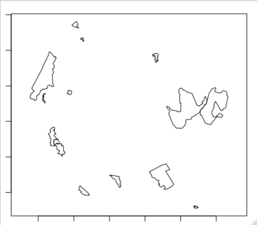
Plotting it I get:

Figure 1

The next steps on your code will throw the next result:

#' location data
x_ <- c(707692, 707589, 707998, 708407, 708916, 709415)
y_ <- c(-3030991,-3031423,-3031640,-3031750,-3032508,-3037158)
mydata <- data.frame(x_, y_)

# transform to trk
trk <-
  mk_track(mydata,
           .x = x_,
           .y = y_,
           crs = CRS("+proj=aea +lat_1=20 +lat_2=-23 +lat_0=0 +lon_0=25 +x_0=0 +y_0=0 +ellps=WGS84 +datum=WGS84 +units=m +no_defs"))

#' calculate home range area
kde_shape_1 <- trk %>%
  hr_kde(., levels = c(0.95))
hr_area(kde_shape_1) / 1e6 # 52.00846

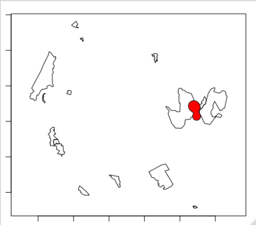
Figure 2

Which I believe is the home area you are defining. Then you do the following:

psf <- qm_rasterToPolygons(kde_shape_1$ud, na.rm = TRUE)

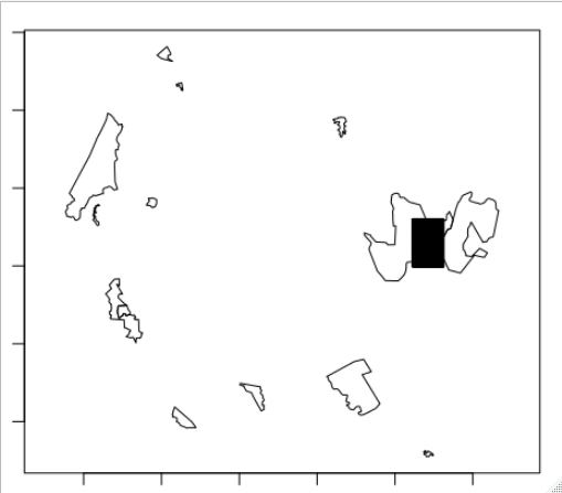
If we plot it, we get:

Figure 3

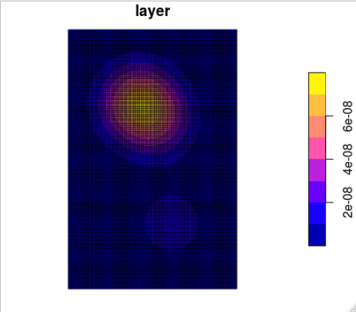
Which I'm guessing is not what you want and might be the origin of your problems. It seems that the function qm_rasterToPolygons uses the whole bounding box of the raster to create a grid of squared polygons (see next figure) rather than creating a polygon with the shape of the home area in figure 2.

Figure 4

If, instead, we use the function hr_isopleths as follows:

test <- hr_isopleths(kde_shape_1)

And we plot it, we obtain the same case as in figure 2 but with the area defined as a polygon with which we can work. Calculating the intersection again as:

intersection <-
  st_intersection(test$geometry, merged_Africa_tranform$geometry)
sum(st_area(intersection)) / 1e6

We now obtain an area of 34.68964 [m^2]

PS: I'm totally out of my element here, so if it is not what you were looking for, just let me know and I'll delete the answer so others are not dissuaded to participate
I'm not quite sure it is what you are looking for but let's give it a try. I run your code, plotting each step so I could analyze graphically the different outputs:

library(tidyverse)
library(amt)
library(sf)
library(spex)

#' load in the protected areas
mycrs <- "+proj=aea +lat_1=20 +lat_2=-23 +lat_0=0 +lon_0=25 +x_0=0 +y_0=0 +datum=WGS84 +units=m +no_defs "

merged_Africa = read_sf("pathToFile/WDPA_Jun2020_SWZ-shapefile-polygons.shp")
st_crs(merged_Africa) <- 4326
merged_Africa_tranform <- st_transform(merged_Africa, mycrs)
st_crs(merged_Africa_tranform)

Plotting it I get:

Figure 1

The next steps on your code will throw the next result:

#' location data
x_ <- c(707692, 707589, 707998, 708407, 708916, 709415)
y_ <- c(-3030991,-3031423,-3031640,-3031750,-3032508,-3037158)
mydata <- data.frame(x_, y_)

# transform to trk
trk <-
  mk_track(mydata,
           .x = x_,
           .y = y_,
           crs = CRS("+proj=aea +lat_1=20 +lat_2=-23 +lat_0=0 +lon_0=25 +x_0=0 +y_0=0 +ellps=WGS84 +datum=WGS84 +units=m +no_defs"))

#' calculate home range area
kde_shape_1 <- trk %>%
  hr_kde(., levels = c(0.95))
hr_area(kde_shape_1) / 1e6 # 52.00846

Figure 2

Which I believe is the home area you are defining. Then you do the following:

psf <- qm_rasterToPolygons(kde_shape_1$ud, na.rm = TRUE)

If we plot it, we get:

Figure 3

Which I'm guessing is not what you want and might be the origin of your problems. It seems that the function qm_rasterToPolygons uses the whole bounding box of the raster to create a grid of squared polygons (see next figure) rather than creating a polygon with the shape of the home area in figure 2.

Figure 4

If, instead, we use the function hr_isopleths as follows:

test <- hr_isopleths(kde_shape_1)

And we plot it, we obtain the same case as in figure 2 but with the area defined as a polygon with which we can work. Calculating the intersection again as:

intersection <-
  st_intersection(test$geometry, merged_Africa_tranform$geometry)
sum(st_area(intersection)) / 1e6

We now obtain an area of 34.68964 [m^2]

added 5 characters in body
Source Link

I'm not quite sure it is what you are looking for but let's give it a try. I run your code, plotting each step so I could analyze graphically the different outputs:

library(tidyverse)
library(amt)
library(sf)
library(spex)

#' load in the protected areas
mycrs <- "+proj=aea +lat_1=20 +lat_2=-23 +lat_0=0 +lon_0=25 +x_0=0 +y_0=0 +datum=WGS84 +units=m +no_defs "

merged_Africa = read_sf("pathToFile/WDPA_Jun2020_SWZ-shapefile-polygons.shp")
st_crs(merged_Africa) <- 4326
merged_Africa_tranform <- st_transform(merged_Africa, mycrs)
st_crs(merged_Africa_tranform)

Plotting it I get:

Figure 1

The next steps on your code will throw the next result:

#' location data
x_ <- c(707692, 707589, 707998, 708407, 708916, 709415)
y_ <- c(-3030991,-3031423,-3031640,-3031750,-3032508,-3037158)
mydata <- data.frame(x_, y_)

# transform to trk
trk <-
  mk_track(mydata,
           .x = x_,
           .y = y_,
           crs = CRS("+proj=aea +lat_1=20 +lat_2=-23 +lat_0=0 +lon_0=25 +x_0=0 +y_0=0 +ellps=WGS84 +datum=WGS84 +units=m +no_defs"))

#' calculate home range area
kde_shape_1 <- trk %>%
  hr_kde(., levels = c(0.95))
hr_area(kde_shape_1) / 1e6 # 52.00846

Figure 2

Which I believe is the home area you are defining. Then you do the following:

psf <- qm_rasterToPolygons(kde_shape_1$ud, na.rm = TRUE)

If we plot it, we get:

Figure 3

Which I'm guessing is not what you want and might be the origin of your problems. It seems that the function qm_rasterToPolygons uses the whole bounding box of the raster to create a grid of squared polygons (see next figure) rather than creating a polygon with the shape of the home area in figure 2.

Figure 4

If, instead, we use the function hr_isopleths as follows:

test <- hr_isopleths(kde_shape_1)

And we plot it, we obtain the same case as in figure 2 but with the area defined as a polygon with which we can work with. Calculating the intersection again as:

intersection <-
  st_intersection(test$geometry, merged_Africa_tranform$geometry)
sum(st_area(intersection)) / 1e6

We now obtain andan area of 34.68964 [m^2]

PS: I'm totally out of my element here, so if it is not what you were looking for, just let me know and I'll delete the answer so others are not dissuaded to participate
I'm not quite sure it is what you are looking for but let's give it a try. I run your code, plotting each step so I could analyze graphically the different outputs:

library(tidyverse)
library(amt)
library(sf)
library(spex)

#' load in the protected areas
mycrs <- "+proj=aea +lat_1=20 +lat_2=-23 +lat_0=0 +lon_0=25 +x_0=0 +y_0=0 +datum=WGS84 +units=m +no_defs "

merged_Africa = read_sf("pathToFile/WDPA_Jun2020_SWZ-shapefile-polygons.shp")
st_crs(merged_Africa) <- 4326
merged_Africa_tranform <- st_transform(merged_Africa, mycrs)
st_crs(merged_Africa_tranform)

Plotting it I get:

Figure 1

The next steps on your code will throw the next result:

#' location data
x_ <- c(707692, 707589, 707998, 708407, 708916, 709415)
y_ <- c(-3030991,-3031423,-3031640,-3031750,-3032508,-3037158)
mydata <- data.frame(x_, y_)

# transform to trk
trk <-
  mk_track(mydata,
           .x = x_,
           .y = y_,
           crs = CRS("+proj=aea +lat_1=20 +lat_2=-23 +lat_0=0 +lon_0=25 +x_0=0 +y_0=0 +ellps=WGS84 +datum=WGS84 +units=m +no_defs"))

#' calculate home range area
kde_shape_1 <- trk %>%
  hr_kde(., levels = c(0.95))
hr_area(kde_shape_1) / 1e6 # 52.00846

Figure 2

Which I believe is the home area you are defining. Then you do the following:

psf <- qm_rasterToPolygons(kde_shape_1$ud, na.rm = TRUE)

If we plot it, we get:

Figure 3

Which I'm guessing is not what you want and might be the origin of your problems. It seems that the function qm_rasterToPolygons uses the whole bounding box of the raster to create a grid of squared polygons (see next figure) rather than creating a polygon with the shape of the home area in figure 2.

Figure 4

If, instead, we use the function hr_isopleths as follows:

test <- hr_isopleths(kde_shape_1)

And we plot it, we obtain the same case as in figure 2 but with the area defined as a polygon we can work with. Calculating the intersection again as:

intersection <-
  st_intersection(test$geometry, merged_Africa_tranform$geometry)
sum(st_area(intersection)) / 1e6

We now obtain and area of 34.68964 [m^2]

PS: I'm totally out of my element here, so if it is not what you were looking for, just let me know and I'll delete the answer so others are not dissuaded to participate
I'm not quite sure it is what you are looking for but let's give it a try. I run your code, plotting each step so I could analyze graphically the different outputs:

library(tidyverse)
library(amt)
library(sf)
library(spex)

#' load in the protected areas
mycrs <- "+proj=aea +lat_1=20 +lat_2=-23 +lat_0=0 +lon_0=25 +x_0=0 +y_0=0 +datum=WGS84 +units=m +no_defs "

merged_Africa = read_sf("pathToFile/WDPA_Jun2020_SWZ-shapefile-polygons.shp")
st_crs(merged_Africa) <- 4326
merged_Africa_tranform <- st_transform(merged_Africa, mycrs)
st_crs(merged_Africa_tranform)

Plotting it I get:

Figure 1

The next steps on your code will throw the next result:

#' location data
x_ <- c(707692, 707589, 707998, 708407, 708916, 709415)
y_ <- c(-3030991,-3031423,-3031640,-3031750,-3032508,-3037158)
mydata <- data.frame(x_, y_)

# transform to trk
trk <-
  mk_track(mydata,
           .x = x_,
           .y = y_,
           crs = CRS("+proj=aea +lat_1=20 +lat_2=-23 +lat_0=0 +lon_0=25 +x_0=0 +y_0=0 +ellps=WGS84 +datum=WGS84 +units=m +no_defs"))

#' calculate home range area
kde_shape_1 <- trk %>%
  hr_kde(., levels = c(0.95))
hr_area(kde_shape_1) / 1e6 # 52.00846

Figure 2

Which I believe is the home area you are defining. Then you do the following:

psf <- qm_rasterToPolygons(kde_shape_1$ud, na.rm = TRUE)

If we plot it, we get:

Figure 3

Which I'm guessing is not what you want and might be the origin of your problems. It seems that the function qm_rasterToPolygons uses the whole bounding box of the raster to create a grid of squared polygons (see next figure) rather than creating a polygon with the shape of the home area in figure 2.

Figure 4

If, instead, we use the function hr_isopleths as follows:

test <- hr_isopleths(kde_shape_1)

And we plot it, we obtain the same case as in figure 2 but with the area defined as a polygon with which we can work. Calculating the intersection again as:

intersection <-
  st_intersection(test$geometry, merged_Africa_tranform$geometry)
sum(st_area(intersection)) / 1e6

We now obtain an area of 34.68964 [m^2]

PS: I'm totally out of my element here, so if it is not what you were looking for, just let me know and I'll delete the answer so others are not dissuaded to participate

added 2 characters in body
Source Link

I'm not quite sure it is what you are looking for but let's give it a try. I run your code, plotting each step so I could analyze graphically the different outputs:

library(tidyverse)
library(amt)
library(sf)
library(spex)

#' load in the protected areas
mycrs <- "+proj=aea +lat_1=20 +lat_2=-23 +lat_0=0 +lon_0=25 +x_0=0 +y_0=0 +datum=WGS84 +units=m +no_defs "

merged_Africa = read_sf("pathToFile/WDPA_Jun2020_SWZ-shapefile-polygons.shp")
st_crs(merged_Africa) <- 4326
merged_Africa_tranform <- st_transform(merged_Africa, mycrs)
st_crs(merged_Africa_tranform)

Plotting it I get:

Figure 1

The next steps on your code will throw the next result:

#' location data
x_ <- c(707692, 707589, 707998, 708407, 708916, 709415)
y_ <- c(-3030991,-3031423,-3031640,-3031750,-3032508,-3037158)
mydata <- data.frame(x_, y_)

# transform to trk
trk <-
  mk_track(mydata,
           .x = x_,
           .y = y_,
           crs = CRS("+proj=aea +lat_1=20 +lat_2=-23 +lat_0=0 +lon_0=25 +x_0=0 +y_0=0 +ellps=WGS84 +datum=WGS84 +units=m +no_defs"))

#' calculate home range area
kde_shape_1 <- trk %>%
  hr_kde(., levels = c(0.95))
hr_area(kde_shape_1) / 1e6 # 52.00846

Figure 2

Which I believe is the home area you are defining. Then you do the following:

psf <- qm_rasterToPolygons(kde_shape_1$ud, na.rm = TRUE)

If we plot it, we get:

Figure 3

Which I'm guessing is not what you want and maymight be the origin of your problems. It seems that the function qm_rasterToPolygons uses the whole bounding box of the raster to create a grid of squared polygons (see next figure) rather than creating a polygon with the shape of the home area in figure 2.

Figure 4

If, instead, we use the function hr_isopleths as follows:

test <- hr_isopleths(kde_shape_1)

And we plot it, we obtain the same case as in figure 2 but with the area defined as a polygon we can work with. Calculating the intersection again as:

intersection <-
  st_intersection(test$geometry, merged_Africa_tranform$geometry)
sum(st_area(intersection)) / 1e6

We now obtain and area of 34.68964 [m^2]

PS: I'm totally out of my element here, so if it is not what you were looking for, just let me know and I'll delete the answer so others are not dissuaded to participate

I'm not quite sure it is what you are looking for but let's give it a try. I run your code, plotting each step so I could analyze graphically the different outputs:

library(tidyverse)
library(amt)
library(sf)
library(spex)

#' load in the protected areas
mycrs <- "+proj=aea +lat_1=20 +lat_2=-23 +lat_0=0 +lon_0=25 +x_0=0 +y_0=0 +datum=WGS84 +units=m +no_defs "

merged_Africa = read_sf("pathToFile/WDPA_Jun2020_SWZ-shapefile-polygons.shp")
st_crs(merged_Africa) <- 4326
merged_Africa_tranform <- st_transform(merged_Africa, mycrs)
st_crs(merged_Africa_tranform)

Plotting it I get:

Figure 1

The next steps on your code will throw the next result:

#' location data
x_ <- c(707692, 707589, 707998, 708407, 708916, 709415)
y_ <- c(-3030991,-3031423,-3031640,-3031750,-3032508,-3037158)
mydata <- data.frame(x_, y_)

# transform to trk
trk <-
  mk_track(mydata,
           .x = x_,
           .y = y_,
           crs = CRS("+proj=aea +lat_1=20 +lat_2=-23 +lat_0=0 +lon_0=25 +x_0=0 +y_0=0 +ellps=WGS84 +datum=WGS84 +units=m +no_defs"))

#' calculate home range area
kde_shape_1 <- trk %>%
  hr_kde(., levels = c(0.95))
hr_area(kde_shape_1) / 1e6 # 52.00846

Figure 2

Which I believe is the home area you are defining. Then you do the following:

psf <- qm_rasterToPolygons(kde_shape_1$ud, na.rm = TRUE)

If we plot it, we get:

Figure 3

Which I'm guessing is not what you want and may be the origin of your problems. It seems that the function qm_rasterToPolygons uses the whole bounding box of the raster to create a grid of squared polygons (see next figure) rather than creating a polygon with the shape of the home area in figure 2.

Figure 4

If, instead, we use the function hr_isopleths as follows:

test <- hr_isopleths(kde_shape_1)

And we plot it, we obtain the same case as in figure 2 but with the area defined as a polygon we can work with. Calculating the intersection again as:

intersection <-
  st_intersection(test$geometry, merged_Africa_tranform$geometry)
sum(st_area(intersection)) / 1e6

We now obtain and area of 34.68964 [m^2]

PS: I'm totally out of my element here, so if it is not what you were looking for, just let me know and I'll delete the answer so others are not dissuaded to participate

I'm not quite sure it is what you are looking for but let's give it a try. I run your code, plotting each step so I could analyze graphically the different outputs:

library(tidyverse)
library(amt)
library(sf)
library(spex)

#' load in the protected areas
mycrs <- "+proj=aea +lat_1=20 +lat_2=-23 +lat_0=0 +lon_0=25 +x_0=0 +y_0=0 +datum=WGS84 +units=m +no_defs "

merged_Africa = read_sf("pathToFile/WDPA_Jun2020_SWZ-shapefile-polygons.shp")
st_crs(merged_Africa) <- 4326
merged_Africa_tranform <- st_transform(merged_Africa, mycrs)
st_crs(merged_Africa_tranform)

Plotting it I get:

Figure 1

The next steps on your code will throw the next result:

#' location data
x_ <- c(707692, 707589, 707998, 708407, 708916, 709415)
y_ <- c(-3030991,-3031423,-3031640,-3031750,-3032508,-3037158)
mydata <- data.frame(x_, y_)

# transform to trk
trk <-
  mk_track(mydata,
           .x = x_,
           .y = y_,
           crs = CRS("+proj=aea +lat_1=20 +lat_2=-23 +lat_0=0 +lon_0=25 +x_0=0 +y_0=0 +ellps=WGS84 +datum=WGS84 +units=m +no_defs"))

#' calculate home range area
kde_shape_1 <- trk %>%
  hr_kde(., levels = c(0.95))
hr_area(kde_shape_1) / 1e6 # 52.00846

Figure 2

Which I believe is the home area you are defining. Then you do the following:

psf <- qm_rasterToPolygons(kde_shape_1$ud, na.rm = TRUE)

If we plot it, we get:

Figure 3

Which I'm guessing is not what you want and might be the origin of your problems. It seems that the function qm_rasterToPolygons uses the whole bounding box of the raster to create a grid of squared polygons (see next figure) rather than creating a polygon with the shape of the home area in figure 2.

Figure 4

If, instead, we use the function hr_isopleths as follows:

test <- hr_isopleths(kde_shape_1)

And we plot it, we obtain the same case as in figure 2 but with the area defined as a polygon we can work with. Calculating the intersection again as:

intersection <-
  st_intersection(test$geometry, merged_Africa_tranform$geometry)
sum(st_area(intersection)) / 1e6

We now obtain and area of 34.68964 [m^2]

PS: I'm totally out of my element here, so if it is not what you were looking for, just let me know and I'll delete the answer so others are not dissuaded to participate

remvoed HTH
Source Link
Vince
  • 20.3k
  • 16
  • 48
  • 65
Loading
added 148 characters in body
Source Link
Loading
added 148 characters in body
Source Link
Loading
added 23 characters in body
Source Link
Loading
Source Link
Loading