I'm not quite sure it is what you are looking for but let's give it a try. I run your code, plotting each step so I could analyze graphically the different outputs:
library(tidyverse)
library(amt)
library(sf)
library(spex)

#' load in the protected areas
mycrs <- "+proj=aea +lat_1=20 +lat_2=-23 +lat_0=0 +lon_0=25 +x_0=0 +y_0=0 +datum=WGS84 +units=m +no_defs "

merged_Africa = read_sf("pathToFile/WDPA_Jun2020_SWZ-shapefile-polygons.shp")
st_crs(merged_Africa) <- 4326
merged_Africa_tranform <- st_transform(merged_Africa, mycrs)
st_crs(merged_Africa_tranform)
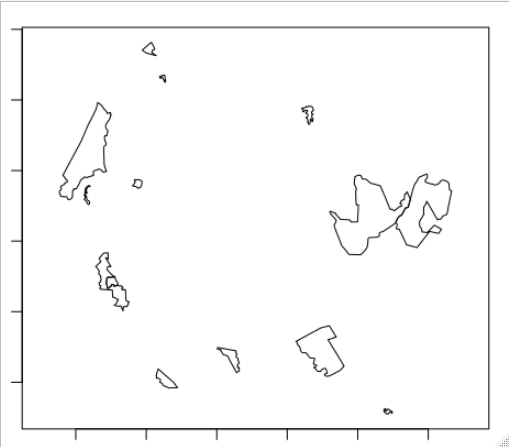
Plotting it I get:
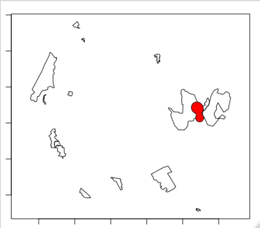
The next steps on your code will throw the next result:
#' location data
x_ <- c(707692, 707589, 707998, 708407, 708916, 709415)
y_ <- c(-3030991,-3031423,-3031640,-3031750,-3032508,-3037158)
mydata <- data.frame(x_, y_)

# transform to trk
trk <-
  mk_track(mydata,
           .x = x_,
           .y = y_,
           crs = CRS("+proj=aea +lat_1=20 +lat_2=-23 +lat_0=0 +lon_0=25 +x_0=0 +y_0=0 +ellps=WGS84 +datum=WGS84 +units=m +no_defs"))

#' calculate home range area
kde_shape_1 <- trk %>%
  hr_kde(., levels = c(0.95))
hr_area(kde_shape_1) / 1e6 # 52.00846
Which I believe is the home area you are defining. Then you do the following:
psf <- qm_rasterToPolygons(kde_shape_1$ud, na.rm = TRUE)
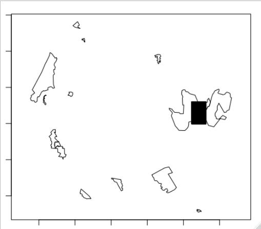
If we plot it, we get:
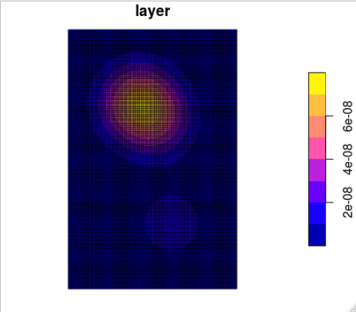
Which I'm guessing is not what you want and might be the origin of your problems. It seems that the function qm_rasterToPolygons uses the whole bounding box of the raster to create a grid of squared polygons (see next figure) rather than creating a polygon with the shape of the home area in figure 2.
If, instead, we use the function hr_isopleths as follows:
test <- hr_isopleths(kde_shape_1)
And we plot it, we obtain the same case as in figure 2 but with the area defined as a polygon with which we can work. Calculating the intersection again as:
intersection <-
  st_intersection(test$geometry, merged_Africa_tranform$geometry)
sum(st_area(intersection)) / 1e6
We now obtain an area of 34.68964 [m^2]


