deleted 166 characters in body
Source Link
Jeffrey Evans
  • 32k
  • 2
  • 48
  • 97

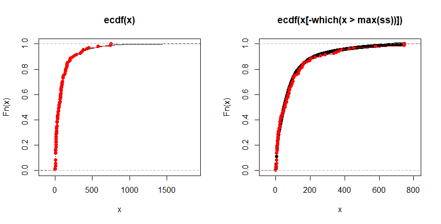
Now, we can clearly see that a random sample, when using the same sample density as our sample data, really does capture sample variation in our population. However, when we look at our sample it is clearly biased away from the upper tail of the population (vertical lines on plot show sample bounds in our data). So, we can say that this is drawn from the population, sharing distributional characteristics with the population but, exhibits a bias. One should note that our random sample is a good representation of the population and in our bootstrap, we applied a KS test comparing our sample against the random sample. We see that length(b[b<0.05]) / length(b) we have 0.30% of our bootstraps that cannot reject the null. This is a significant result in proving that, aside from the bias, we have a good representation of the population distribution. If we look at the empirical cumulative distribution function we see that the sample and population distributions are very well matched, except for missing that upper tail. If we truncate the distribution they are almost exact.

par(mfrow=c(1,2))
  plot(ecdf(x),)
 pch=20   plot(ecdf(ss), col="red", add=TRUE) 
  plot(ecdf(x[-which(x > max(ss))]))
    plot(ecdf(ss), col="red", add=TRUE) 

CDFecdf

Now, we can clearly see that a random sample, when using the same sample density as our sample data, really does capture sample variation in our population. However, when we look at our sample it is clearly biased away from the upper tail of the population (vertical lines on plot show sample bounds in our data). So, we can say that this is drawn from the population, sharing distributional characteristics with the population but, exhibits a bias. One should note that our random sample is a good representation of the population and in our bootstrap, we applied a KS test comparing our sample against the random sample. We see that length(b[b<0.05]) / length(b) we have 0.30% of our bootstraps that cannot reject the null. This is a significant result in proving that, aside from the bias, we have a good representation of the population distribution. If we look at the empirical cumulative distribution function we see that the sample and population distributions are well matched, except for missing that upper tail.

plot(ecdf(x), pch=20, col="red")
  plot(ecdf(ss), add=TRUE)

CDF

Now, we can clearly see that a random sample, when using the same sample density as our sample data, really does capture sample variation in our population. However, when we look at our sample it is clearly biased away from the upper tail of the population (vertical lines on plot show sample bounds in our data). So, we can say that this is drawn from the population, sharing distributional characteristics with the population but, exhibits a bias. One should note that our random sample is a good representation of the population and in our bootstrap, we applied a KS test comparing our sample against the random sample. We see that length(b[b<0.05]) / length(b) we have 0.30% of our bootstraps that cannot reject the null. This is a significant result in proving that, aside from the bias, we have a good representation of the population distribution. If we look at the empirical cumulative distribution function we see that the sample and population distributions are very well matched, except for missing that upper tail. If we truncate the distribution they are almost exact.

par(mfrow=c(1,2))
  plot(ecdf(x))
    plot(ecdf(ss), col="red", add=TRUE) 
  plot(ecdf(x[-which(x > max(ss))]))
    plot(ecdf(ss), col="red", add=TRUE) 
ecdf

deleted 166 characters in body
Source Link
Jeffrey Evans
  • 32k
  • 2
  • 48
  • 97

In ArcGIS you can pull summary statistics directly from the attribute table of your subsamplesample. You can also see the statistics associated with a raster by simply right clicking on the raster in the TOC, selecting properties and going to the source tab. However, I would build statistics first and set the skip value to 1. This will ensure that you are returning statistics for the entire raster. Now, you can just compare your sample statistics to your raster. Your sample mean/median should match the central tendency and the variance should match the spread.

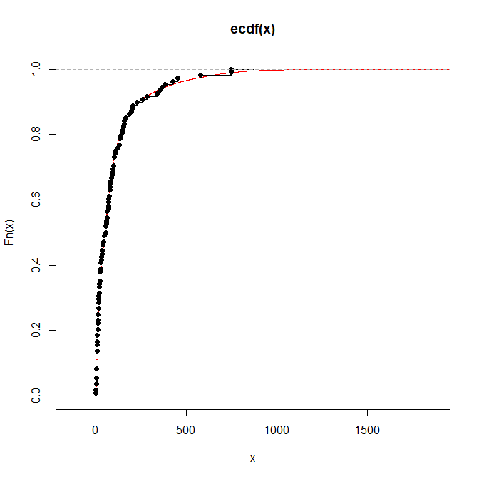
Now, we can clearly see that a random sample, when using the same sample density as our sample data, really does capture sample variation in our population. However, when we look at our sample it is clearly biased away from the upper tail of the population (vertical lines on plot show sample bounds in our data). So, we can say that this is drawn from the population, sharing distributional characteristics with the population but, exhibits a bias. One should note that our random sample is a good representation of the population and in our bootstrap, we applied a KS test comparing our sample against the random sample. We see that length(b[b<0.05]) / length(b) we have 0.30% of our bootstraps that cannot reject the null. This is a significant result in proving that, aside from the bias, we have a good representation of the population distribution. If we look at the empirical cumulative distribution function we see that the sample and population distributions are well matched, except for missing that upper tail. So, when we compare the population to the CDF(sample) the p-value is suddenly < 0.00000000000000022 due to the mismatched variances.

ks.test(x, ecdf(ss))

plot(ecdf(x), pch=20, col="red")
  plot(ecdf(ss), add=TRUE)

In ArcGIS you can pull summary statistics directly from the attribute table of your subsample. You can also see the statistics associated with a raster by simply right clicking on the raster in the TOC, selecting properties and going to the source tab. However, I would build statistics first and set the skip value to 1. This will ensure that you are returning statistics for the entire raster. Now, you can just compare your sample statistics to your raster. Your sample mean/median should match the central tendency and the variance should match the spread.

Now, we can clearly see that a random sample, when using the same sample density as our sample data, really does capture sample variation in our population. However, when we look at our sample it is clearly biased away from the upper tail of the population (vertical lines on plot show sample bounds in our data). So, we can say that this is drawn from the population, sharing distributional characteristics with the population but, exhibits a bias. One should note that our random sample is a good representation of the population and in our bootstrap, we applied a KS test comparing our sample against the random sample. We see that length(b[b<0.05]) / length(b) we have 0.30% of our bootstraps that cannot reject the null. This is a significant result in proving that, aside from the bias, we have a good representation of the population distribution. If we look at the empirical cumulative distribution function we see that the sample and population distributions are well matched, except for missing that upper tail. So, when we compare the population to the CDF(sample) the p-value is suddenly < 0.00000000000000022 due to the mismatched variances.

ks.test(x, ecdf(ss))

plot(ecdf(x), pch=20, col="red")
  plot(ecdf(ss), add=TRUE)

In ArcGIS you can pull summary statistics directly from the attribute table of your sample. You can also see the statistics associated with a raster by simply right clicking on the raster in the TOC, selecting properties and going to the source tab. However, I would build statistics first and set the skip value to 1. This will ensure that you are returning statistics for the entire raster. Now, you can just compare your sample statistics to your raster. Your sample mean/median should match the central tendency and the variance should match the spread.

Now, we can clearly see that a random sample, when using the same sample density as our sample data, really does capture sample variation in our population. However, when we look at our sample it is clearly biased away from the upper tail of the population (vertical lines on plot show sample bounds in our data). So, we can say that this is drawn from the population, sharing distributional characteristics with the population but, exhibits a bias. One should note that our random sample is a good representation of the population and in our bootstrap, we applied a KS test comparing our sample against the random sample. We see that length(b[b<0.05]) / length(b) we have 0.30% of our bootstraps that cannot reject the null. This is a significant result in proving that, aside from the bias, we have a good representation of the population distribution. If we look at the empirical cumulative distribution function we see that the sample and population distributions are well matched, except for missing that upper tail.

plot(ecdf(x), pch=20, col="red")
  plot(ecdf(ss), add=TRUE)
added 469 characters in body
Source Link
Jeffrey Evans
  • 32k
  • 2
  • 48
  • 97

Now, we can clearly see that a random sample, when using the same sample density as our sample data, really does capture sample variation in our population. However, when we look at our sample it is clearly biased away from the upper tail of the population (vertical lines on plot show sample bounds in our data). So, we can say that this is drawn from the population, sharing distributional characteristics with the population but, exhibits a bias. One should note that our random sample is a good representation of the population and in our bootstrap, we applied a KS test comparing our sample against the random sample. We see that length(b[b<0.05]) / length(b) we have 0.30% of our bootstraps that cannot reject the null. This is a significant result in proving that, aside from the bias, we have a good representation of the population distribution. If we look at the empirical cumulative distribution function we see that the sample and population distributions are well matched, except for missing that upper tail. So, when we compare the population to the CDF(sample) the p-value is suddenly < 0.00000000000000022 due to the mismatched variances.

ks.test(x, ecdf(ss))

plot(ecdf(x), pch=20, col="red")
  plot(ecdf(ss), add=TRUE)

CDF

Now, we can clearly see that a random sample, when using the same sample density as our sample data, really does capture sample variation in our population. However, when we look at our sample it is clearly biased away from the upper tail of the population (vertical lines on plot show sample bounds in our data). So, we can say that this is drawn from the population, sharing distributional characteristics with the population but, exhibits a bias. One should note that our random sample is a good representation of the population and in our bootstrap, we applied a KS test comparing our sample against the random sample. We see that length(b[b<0.05]) / length(b) we have 0.30% of our bootstraps that cannot reject the null. This is a significant result in proving that, aside from the bias, we have a good representation of the population distribution.

Now, we can clearly see that a random sample, when using the same sample density as our sample data, really does capture sample variation in our population. However, when we look at our sample it is clearly biased away from the upper tail of the population (vertical lines on plot show sample bounds in our data). So, we can say that this is drawn from the population, sharing distributional characteristics with the population but, exhibits a bias. One should note that our random sample is a good representation of the population and in our bootstrap, we applied a KS test comparing our sample against the random sample. We see that length(b[b<0.05]) / length(b) we have 0.30% of our bootstraps that cannot reject the null. This is a significant result in proving that, aside from the bias, we have a good representation of the population distribution. If we look at the empirical cumulative distribution function we see that the sample and population distributions are well matched, except for missing that upper tail. So, when we compare the population to the CDF(sample) the p-value is suddenly < 0.00000000000000022 due to the mismatched variances.

ks.test(x, ecdf(ss))

plot(ecdf(x), pch=20, col="red")
  plot(ecdf(ss), add=TRUE)

CDF

added 129 characters in body
Source Link
Jeffrey Evans
  • 32k
  • 2
  • 48
  • 97
Loading
Source Link
Jeffrey Evans
  • 32k
  • 2
  • 48
  • 97
Loading