How to find if a non-random subsample of a raster is significantly different from the raster using ArcGIS 10.7

Question

I am attempting to find a way to test if the values from a non-random sample of my raster values is significantly different from the raster values as a whole. In this case, I have extracted values for land surface temperature to the known locations of people suffering heat strokes using ArcGIS 10.7.1. I want to know whether these locations' temperatures are distinct from the landscape as a whole. Although using Arc, I could use R if needed.

Answer 1

This is a bit of a tricky question. There is a simple answer and a correct one. Which path you choose should be dictated by your motivation and need. If this is just meant to be a gut check you can simply compare the mean, median and variance of the sample to the raster moments.

In ArcGIS you can pull summary statistics directly from the attribute table of your sample. You can also see the statistics associated with a raster by simply right clicking on the raster in the TOC, selecting properties and going to the source tab. However, I would build statistics first and set the skip value to 1. This will ensure that you are returning statistics for the entire raster. Now, you can just compare your sample statistics to your raster. Your sample mean/median should match the central tendency and the variance should match the spread.

Now, the "correct" way is what you do if you are needing to meet a "burden of proof" say, for publication. Unfortunately, there is no path forward for doing this type of analysis in ESRI software so, you are stuck with a statistical software (Stata, Matlab, R, SAS, Python, ...). I will give examples using R.

Lets first add some data to use in our analysis. We will treat this as our known sample and population (raster). The raster is a DEM of Cuba which we then take a systematic sample of, well knowing the spatial bias associated with this type of sample.

library(raster)
library(sp)

r <- getData("alt", country='CUB', mask=TRUE)
  r[r < 0] <- 0
s <- sampleRegular(r, size=500, sp=TRUE)
  s <- s[-which(is.na(s@data[,1])),]

plot(r)
  points(s, pch=20, cex=0.75)

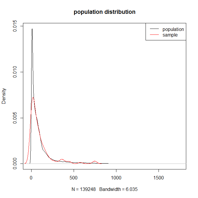
To start our analysis we create a vector of our raster population (x) and one of our sample (ss), display some some summary statistics and plot the two probability density functions (distributions).

x <- r[!is.na(r)]
  x[x < 0] <- 0
ss <- as.numeric(s@data[,1])

summary(x)
summary(ss)

plot(density(x), main="population distribution")
  lines(density(ss), col="red")
    legend("topright", legend=c("population", "sample"),
           lty=c(1,1), col=c("black","red"))

We can qualitatively say that these two distributions look similar and have similar means but, can we quantitatively prove it? If we look at some other moments, we are missing the upper tail and the variances are very mismatched (22442.28, 19627.35) showing that the sample is not capturing the population variation.

There are many tests that could be leveraged here, most familiar is likely the t-test. However, there are well known issues associated with non-normality and large sample size that can make parametric tests questionable. Fortunately, there are test that can handle non-normality and unequal (large) sample sizes.

Since we can not assume normality we can leverage the "one sample Kolmogorov-Smirnov" statistic for testing if a variable follows a given expected distribution. The KS test is nonparametric and does not assume equal variance so, is good for this type of comparison. If we were comparing against ranks (eg., landcover) the Kruskal-Wallis would come into play.

ks.test(x, ss)

Here, our p-value is p=0.99 so, we can reject the null. However, what about that variance issue.

First we can use a Kolmogorov-Smirnov test with a random sample to test for sample convergence (eg., how large of a random sample do we need to capture population variation).

b <-lapply(round(length(x)*c(0.01, 0.05, 0.10, 0.25, 0.30),0), 
            function(i) {
            xs <- x[sample(1:length(x), i)]
            return(
            c(summary(xs), variance=var(xs), 
            p.value=suppressWarnings(ks.test(x, xs)$p.value)
            ))
  })
names(b) <- paste0("n=", round(length(x)*c(0.01, 0.05, 0.10, 0.25, 0.30),0))
  print(b)
    c(summary(x), variance=var(x))

This test tells us that even relatively small random sample sizes (p>=0.01) can represent the sample distribution and population variation. Note the convergence of the variance.

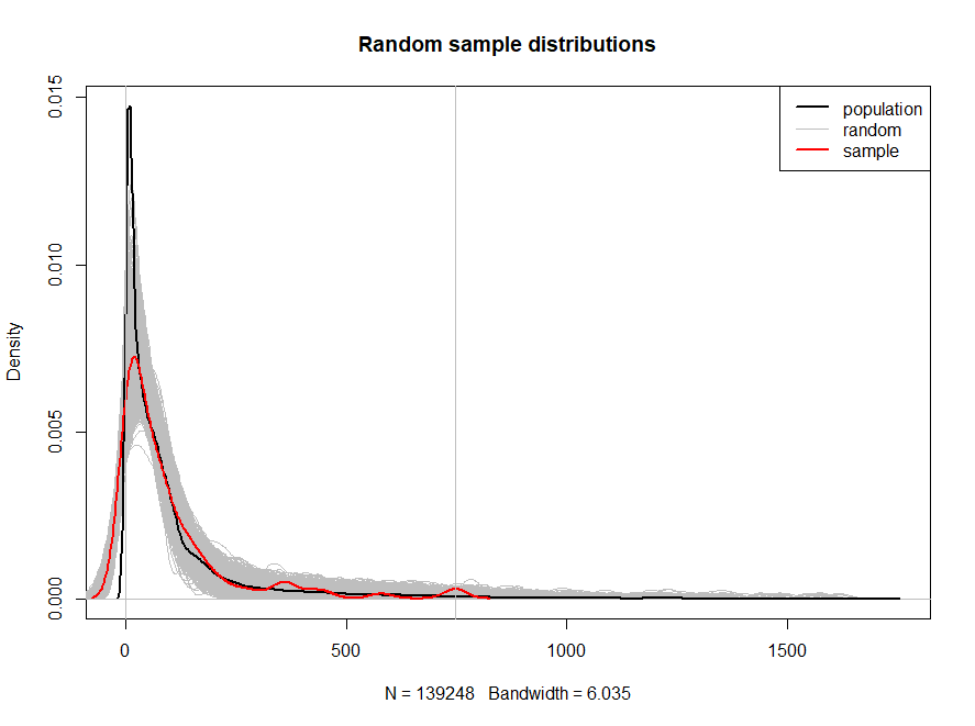
Now, we know that a random sample is a somewhat stable representation of the population so, let's test it using a random sample in a bootstrap.

plot(density(x), type="n", main="Random sample distributions")
  b <- unlist(lapply(1:999, function(i) {
              xs <- x[sample(1:length(x), nrow(s))]
              lines(density(xs), lwd=0.75, col="grey")
              return(suppressWarnings(ks.test(ss, xs)$p.value))
  })) 
  
lines(density(x), col="black", lwd=2)  
lines(density(ss), col="red", lwd=2)
  abline(v=c(min(ss), max(ss)), col="grey")
  legend("topright", legend=c("population", "random", "sample"),
         lty=c(1,1,1), lwd=c(2,1,2), 
         col=c("black", "grey", "red"))  

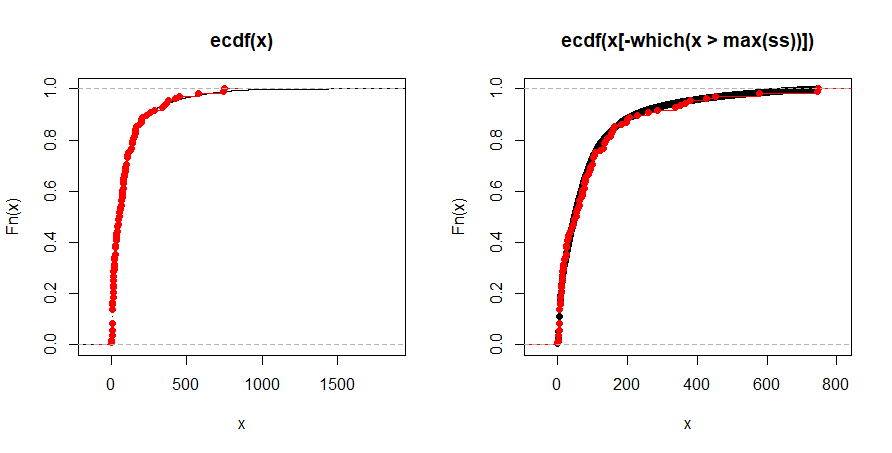
Now, we can clearly see that a random sample, when using the same sample density as our sample data, really does capture sample variation in our population. However, when we look at our sample it is clearly biased away from the upper tail of the population (vertical lines on plot show sample bounds in our data). So, we can say that this is drawn from the population, sharing distributional characteristics with the population but, exhibits a bias. One should note that our random sample is a good representation of the population and in our bootstrap, we applied a KS test comparing our sample against the random sample. We see that length(b[b<0.05]) / length(b) we have 0.30% of our bootstraps that cannot reject the null. This is a significant result in proving that, aside from the bias, we have a good representation of the population distribution. If we look at the empirical cumulative distribution function we see that the sample and population distributions are very well matched, except for missing that upper tail. If we truncate the distribution they are almost exact.

par(mfrow=c(1,2))
  plot(ecdf(x))
    plot(ecdf(ss), col="red", add=TRUE) 
  plot(ecdf(x[-which(x > max(ss))]))
    plot(ecdf(ss), col="red", add=TRUE)