How do you get GPM IMERG data in R?

Question

I want to get proper GPM IMERG data with variables including time in R and work with it. I used "https://disc.gsfc.nasa.gov/" and got the link list in txt file. I don't know what to do from here. Could someone give an idea?

Answer 1

Terra can open IMERG rasters, but these files don't have CRS and are flipped, so you must correct them before computing or implementing any analysis. In this case, I list the files inside a folder, then I iterate through files opening, correcting the X Y dimension (transposing the file), adding the CRS, and saving the result to a list):

library(terra)

fnames <- list.files(pattern = 'IMERG')

rlist <- list()

for (i in seq_along(fnames)) {
  r = rast(fnames[i])
  r = trans(r)
  ext(r) = c(-180,180,-90,90)
  crs(r) = "epsg:4326"
  rlist[[i]] = r
}

Then, you can perform any arithmetic operation or zonal stats or whatever you want to achieve.

If you need only one band, the process is faster:

rlist <- list()

for (i in seq_along(fnames)) {
  r = rast(fnames[i])['precipitationCal']
  r = trans(r)
  ext(r) = c(-180,180,-90,90)
  crs(r) = "epsg:4326"
  rlist[[i]] = r
}

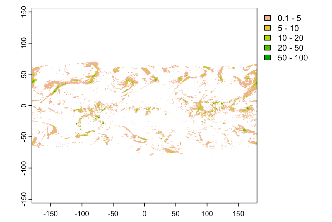
plot(app(rast(rlist), sum), type = "interval",
     breaks = c(0.1,5,10,20,50,100))

I also post the same process with python using a custom function:

import rioxarray as rioxr

def load_imerg(file, var):
  da = rioxr.open_rasterio(file, engine='h5netcdf')
  da = da[0][var]
  return da.assign_coords({"x": (da.x / 10) - 90}) \
      .assign_coords({"y": (da.y / 10) - 180}) \
      .transpose('band', 'x', 'y') \
      .rio.write_crs(4326) \
      .rename({'x': 'y', 'y': 'x'})

You can loop using this function saving the results to a list as well.

I'm working with 30" product, so I found Python solution faster than R for doing the same task over thousands files.

Answer 2

I built a program without using TERRA library and it works!

rm(list = ls())

# Load the necessary libraries
library(ncdf4)
library(lattice)
library(latticeExtra)
library(colorspace)
library(dplyr)
library(RColorBrewer)
library(cptcity)
library(grid)
library(gridExtra)
library(raster)

# Define the path to the NetCDF file
nc_path <- "/home/decker/imerge/imerge/DEC/dec.nc"

# Open the NetCDF file
nc_data <- nc_open(nc_path)

# Extract the latitude and longitude variables
lat <- ncvar_get(nc_data, "lat")
lon <- ncvar_get(nc_data, "lon")

# Close the NetCDF file
nc_close(nc_data)

# Load the raster file with terra
r <- rast(nc_path)

# Select the specific precipitation band
r_precip <- r[['precipitationCal_49']]  # Adjust the band number as necessary

# Transpose the raster to correct the orientation
r_precip <- t(r_precip)

# Flip the raster to correct the north-south orientation
r_precip <- flip(r_precip, direction = "vertical")

# Flip the raster to correct the east-west orientation
r_precip <- flip(r_precip, direction = "horizontal")

# Adjust the raster extent using the extracted coordinates
ext(r_precip) <- c(min(lon), max(lon), min(lat), max(lat))

# Define the CRS
crs(r_precip) <- "epsg:4326"

# Define the color palette
corDegrade <- colorRampPalette(c('ivory3', 'dodgerblue', 'cadetblue', 'yellowgreen',
                                 'yellow', 'orange', 'darkorange2', 'red2', 'red4'))
shape <- shapefile('/home/decker/Dropbox/academico_2023/shapes/BoliviaShape/BOL_adm1.shp')

# Generate the plot using spplot
trmm <- spplot(r_precip,
               xlab="Longitude", ylab="Latitude",
               colorkey=TRUE,
               scales=list(draw=TRUE),
               main="Precipitation - TRMM3B42",
               col.regions=corDegrade) +
  layer(sp.lines(shape, lwd = 1, fill = "transparent", col = 'black'))

# Display the plot
print(trmm)