Aggregation with st_buffer in EPSG 4326 versus other CRS

Question

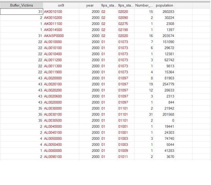
I am trying to find the total sum of homicides within a 1km buffer around each police agency where the homicides were reported. I tried the R code below and it seemed to produce numbers that made sense:

crime<- read_dta("UCR Homicides Total Count 1976-2020 All Victims April12.dta")
state_fips <- read.csv("us-state-fips.csv", header=TRUE)
US_counties <- counties(state = state_fips$st, class="sf")
US_counties <- st_transform(US_counties, crs=4326)


crime$latitude <- as.numeric(crime$latitude)
crime$longitude <- as.numeric(crime$longitude)
crime<-na.omit(crime)

# Do lapply to filter crime data into separate years

crime_years <- lapply(2000:2018, function(x) {filter(crime, year==x)})
# Buffer distance of 1 km
aggregate_buffer_1km <- function(x) {
  crime_sf <- st_as_sf(x, coords= c("longitude", "latitude"))
  st_crs(crime_sf) <- st_crs(US_counties)
  crime_buffer <-st_buffer(crime_sf, dist=1000)
  crime_buffer_number <-aggregate(crime_sf[, "Number_Victims"], crime_buffer, sum) 
  crime_buffer_data <- crime_buffer_number %>%
    st_drop_geometry() %>%
    dplyr::rename(Buffer_Victims = Number_Victims)
  crime_data <- st_drop_geometry(crime_sf)
  crime_buffer_data_final_1km <- data.frame(crime_buffer_data, crime_data)
  return(crime_buffer_data_final_1km)
}

aggregated_crime_data_list_1km <- lapply(crime_years, aggregate_buffer_1km)

The above code produced the following data:

Unfortunately I then read some conflicting information about buffer units in 4326 CRS in R. This post: https://stackoverflow.com/questions/54754277/what-unit-is-the-dist-argument-in-st-buffer-set-to-by-default suggested that I reproject the data into a CRS that has metric units and later convert everything back to 4326. This post : https://stackoverflow.com/questions/73489910/create-buffers-in-km-units-for-global-point-dataset-in-r suggested my earlier code was correct.

To check I wrote the following code to reproject the data to EPSG 5070 which uses metric units and then after buffering reproject back to 4326.

crime<- read_dta("UCR Homicides Total Count 1976-2020 All Victims April12.dta")
state_fips <- read.csv("us-state-fips.csv", header=TRUE)
US_counties <- counties(state = state_fips$st, class="sf")
US_counties <- st_transform(US_counties, crs=5070)

crime$latitude <- as.numeric(crime$latitude)
crime$longitude <- as.numeric(crime$longitude)
crime<-na.omit(crime)

# Do lapply to filter crime data into separate years

crime_years <- lapply(2000:2018, function(x) {filter(crime, year==x)})
# Buffer distance of 1 km
aggregate_buffer_1km <- function(x) {
  crime_sf <- st_as_sf(x, coords= c("longitude", "latitude"))
  st_crs(crime_sf) <- st_crs(US_counties)
  crime_buffer <-st_buffer(crime_sf, dist=1000)
  crime_sf <- st_transform(crime_sf, 4326)
  crime_buffer <- st_transform(crime_buffer, 4326)
  crime_buffer_number <-aggregate(crime_sf[, "Number_Victims"], crime_buffer, sum) 
  crime_buffer_data <- crime_buffer_number %>%
    st_drop_geometry() %>%
    dplyr::rename(Buffer_Victims = Number_Victims)
  crime_data <- st_drop_geometry(crime_sf)
  crime_buffer_data_final_1km <- data.frame(crime_buffer_data, crime_data)
  return(crime_buffer_data_final_1km)
}

aggregated_crime_data_list_1km <- lapply(crime_years, aggregate_buffer_1km)

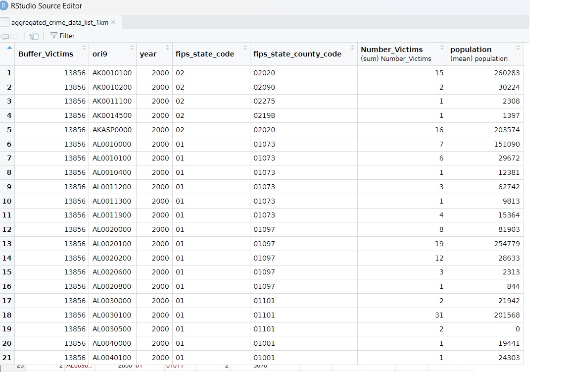
Now my data looks seriously wrong:

I am not sure which is the right approach. I don't understand why the first approach which seems wrong to me according to the advice given online seemed to produce numbers that look right but the second approach seems to produce numbers that look way off. Can anyone shed light on the way to accomplish this task?

Answer 1

At this point you transform US Counties to 5070:

US_counties <- st_transform(US_counties, crs=5070)

But at this point you assign the CRS of the counties to that of the crimes:

  crime_sf <- st_as_sf(x, coords= c("longitude", "latitude"))
  st_crs(crime_sf) <- st_crs(US_counties)

but the crime coordinates at this point are still in lat-long. You need to assign a lat-long CRS to the crime locations, (epsg 4326) and then st_transform them to 5070 (or st_crs(US_counties)).

You can do the assign in st_as_sf when creating sf objects from data frames:

crime_sf = st_as_sf(x, coords=c("longitude","latitude"), crs=4326)
crime_sf = st_transform(crime_sf, st_crs(US_counties))

should work, not tested.