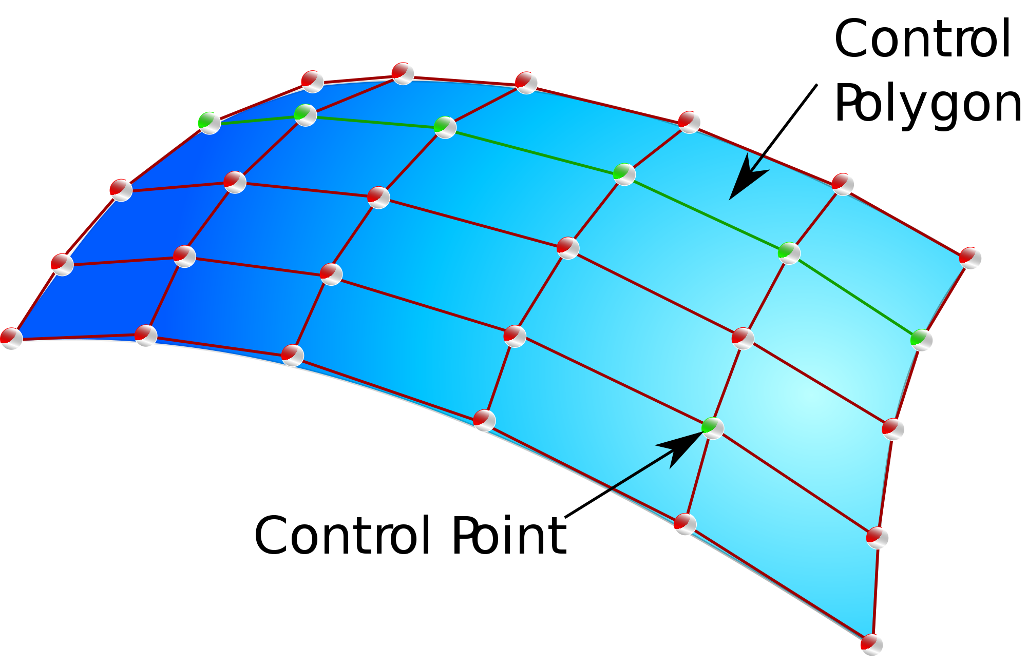
I have a curve surface (example is attached). Each node has its own coordinate in geographic system (longitude,latitude and depth). I want to calculate a distance between two nodes (from the one on the upper left to another on the lower right). However, I want it a distance that follows curve of the surface (not a shortest distance).
2 Answers
As you have a point data set, one approach consists in (1) fitting a surface model, (2) use the model to sample your trajectory and (3) compute the lenght of your trajectory.
Here is an example with python based on scipy that computes the surface trajectory lenght between two points A and B:
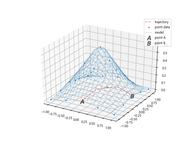
I used a multivariate gaussian model (scipy.stats.multivariate_normal) to generate a grid of 5x5 points as data set for this example (blue dots on the picture).
For step 1, I fitted a a surface model (scipy.interpolate.CloughTocher2DInterpolator) reprensented by the blue wireframe on the figure.
Then, for step 2, i used the same model to generate the red trajectory from 30 xy coordinates linearly sampled between A and B. This leads to 29 trajectory segments.
Step 3 consists in summing each length of the trajectory segments computed by the pythagore formula (lenght = sqrt(dxy**2 + dz**2)).
Of course, the result of such approach is conditionned to the density of your point dataset and the appropriateness of your interpolation model.
Code
from mpl_toolkits.mplot3d import Axes3D
import matplotlib.pyplot as plt
import numpy as np
from scipy.stats import multivariate_normal
from scipy import interpolate


# 0. Create a point xyz data set
#-------------------------------

# Generate x and y (5,5) grids

xx, yy = np.mgrid[-1.0:1.0:5j, -1.0:1.0:5j]

# array of coordinates.
xy = np.column_stack([xx.flat, yy.flat])

# generate 2d gaussian point data

mu = np.array([0.0, 0.0])
sigma = np.array([.5, .5])
covariance = np.diag(sigma**2)
z = multivariate_normal.pdf(xy, mean=mu, cov=covariance)

# Reshape back to a (5, 5) grid.
zz = z.reshape(xx.shape)

# 1. Create a surface model from the point data set
#--------------------------------------------------

# fit model

model = interpolate.CloughTocher2DInterpolator(xy, z)

# generate a new grid with higher resolution (20,20)

xnew, ynew = np.mgrid[-1.0:1.0:20j, -1.0:1.0:20j]

# conversion to array of coordinates

xynew = np.column_stack([xnew.flat, ynew.flat])

# predict z for the new grid

znew = model(xynew).reshape(20,20)

# 2. Use the model to calculate trajectory
#-----------------------------------------

# select two points from xy coordinates

pt1 = np.append(xy[10], z[10])
pt2 = np.append(xy[22], z[22])

# create xy trajectory between points

nstep = 30 # number of point to define the trajectory

x_traj = np.linspace(pt1[0], pt2[0], nstep)
y_traj = np.linspace(pt1[1], pt2[1], nstep)

# get z from model

z_traj = model(zip(x_traj, y_traj))

# 3. Compute trajectory length
#-----------------------------

# euclidean distance in the xy plane between pt1 and pt2

dist_xy = np.linalg.norm(pt1[:-1] - pt2[:-1])

# difference of elevation along trajectory

z_diff = np.diff(z_traj)

# step distance

step = dist_xy /(nstep - 1)

# xyz trajectory length

dist_xyz = np.sum(np.sqrt(step**2 + z_diff**2))

print dist_xyz # <--- RESULT

# Plot results
#-------------

plt.rcParams['font.family'] = 'Segoe UI'
plt.rcParams['font.size'] = 8.

fig = plt.figure()

ax = fig.add_subplot(111, projection='3d')
ax.scatter(xx, yy, zz, alpha=0.8, s=5., label='point data')
ax.plot_wireframe(xnew, ynew, znew, alpha=0.2, label='model')
ax.scatter(pt1[0],pt1[1], pt1[2], color='k', alpha=0.5, marker='$A$', s=100., label='point A')
ax.scatter(pt2[0],pt2[1], pt2[2], color='k', alpha=0.5, marker='$B$', s=100., label='point B')
ax.plot(x_traj, y_traj, z_traj, 'r--', label='trajectory', alpha=0.5)

ax.legend()
plt.show()
It's just due to the depth. Actually this cirve surface covers only 100 by 200 km area. I was initially using vincenty distance but soon realized that it is not what I want because I am expect the curve distance due to the depth.
-
This should really be a comment, or even an edit as it sounds like you are the author of this question. If that's the case, you should use your original account and merge this one with it if necessary. Commented Feb 10, 2016 at 13:07


