Inverse distance weighting variable search radius based on third variable [closed]

Question

I am trying to perform inverse distance weighting (and possibly kriging), but want to base the search radius on a third variable:

• high population density -> small search radius
• low population density -> big search radius

I have been looking at various examples in ArcGIS, R's gstat and Python, but cannot seem to find a solution. In all solution, I can only vary the search radius based on the number of points found.

In order or preference, I am looking for a solution in Python, R or ArcGIS. Any help?

Answer 1

As far as I understand your question, I think you have to make two Inverse Distance Weighting interpolations: one using the small search radius for the high population density data and the other with a big search radius using the low population density data.

I give you a reproducible example in R using the data("meuse"). Almost all the code is commented for help and guidance. You will find three IDW examples: 1. all the data, 2. high values of Zinc with small search radius and 3. low values of Zinc with big search radius.

Note 1: in R using the function idw() from the package gstat you can vary the search radius with the maxdist option.

# Load libraries and data -------------------------------------------------

# Libraries
library("gstat")
library("sp")

# Load Meuse dataset example
data("meuse")

# Create new SpatialPointsDataFrame object
meuseSPDF <- meuse
coordinates(meuseSPDF) <- c("x","y")

# Apply projection
proj4string(meuseSPDF) <- CRS("+init=epsg:28992")

# Explore data ------------------------------------------------------------

# Interactive Map of meuse dataset
# To install mapview library: devtools::install_github("environmentalinformatics-marburg/mapview", ref = "develop")

mapview::mapView(meuseSPDF)

# Bubbleplot of Zinc concentrations
bubble(meuseSPDF, zcol = "zinc", main = "Zinc")

# Explore Zinc values frequency distribution
hist(meuseSPDF$zinc, breaks = seq(100, 2000, by = 100), col = "black", border = "white", xlab = "Zinc concentrations (ppm)", main = "Histogram")

# Geometric Interpolation of Zinc: Inverse Distance Weighthing (ID) -------

# Define (arbitrary) high Zinc concentrations above 500 ppm
highZinc <- meuseSPDF[which(meuseSPDF$zinc > 500),]

# Define (arbitrary) low Zinc concentrations below or equal to 500 ppm
lowZinc <- meuseSPDF[which(meuseSPDF$zinc <= 500),]

# Interpolate
# Make grid (where to interpolate, same extent as the SpatialPointsdataFrame object and 1000 arbitrary points) 

# All
newdataZinc <- spsample(x = Zinc, type = "regular", n = 1000)
searchRadius <- 150
zn.idw <- idw(formula = zinc ~ 1, locations = meuseSPDF, newdata = newdataZinc, maxdist = searchRadius)

# High zinc
newdataHighZinc <- spsample(x = highZinc, type = "regular", n = 1000)
searchRadiusSmall <- 100
znHigh.idw <- idw(formula = zinc ~ 1, locations = highZinc, newdata = newdataHighZinc, maxdist = searchRadiusSmall)

# Low zinc
newdataLowZinc <- spsample(x = lowZinc, type = "regular", n = 1000)
searchRadiusBig <- 200
znLow.idw <- idw(formula = zinc ~ 1, locations = lowZinc, newdata = newdataLowZinc, maxdist = searchRadiusBig)

# Plot predicted values
spplot(zn.idw, zcol = "var1.pred") # all
spplot(znHigh.idw, zcol = "var1.pred") # high
spplot(znLow.idw, zcol = "var1.pred") # low

# Convert predicted values to grid
zn.idw.grid <- SpatialPixelsDataFrame(points = zn.idw, data = zn.idw@data) # all
znHigh.idw.grid <- SpatialPixelsDataFrame(points = znHigh.idw, data = znHigh.idw@data) # high
znLow.idw.grid <- SpatialPixelsDataFrame(points = znLow.idw, data = znLow.idw@data) # low

# Plot predicted grid values
spplot(zn.idw.grid, zcol = "var1.pred", at = seq(0, 2000, 100)) # all
spplot(znHigh.idw.grid, zcol = "var1.pred", at = seq(0, 2000, 100)) # high
spplot(znLow.idw.grid, zcol = "var1.pred", at = seq(0, 2000, 100)) # low

# Interactive Map of predicted grid values  -------------------------------

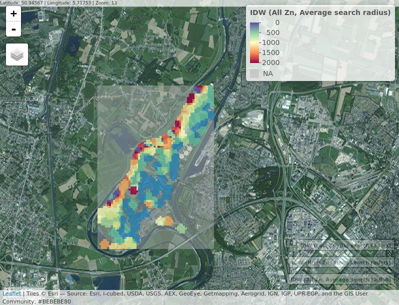
(allMap <- mapview::mapView(raster::raster(zn.idw.grid), at = seq(from = 0, to = 2000, by = 100), col.regions = rev(RColorBrewer::brewer.pal(11, "Spectral")), legend = TRUE, layer.name = "IDW (All Zn, Average search radius)", alpha.regions = 0.8))

(highMap <- mapview::mapView(raster::raster(znHigh.idw.grid), at = seq(from = 0, to = 2000, by = 100), col.regions = rev(RColorBrewer::brewer.pal(11, "Spectral")), legend = TRUE, layer.name = "IDW (High Zn, Small search radius)", alpha.regions = 0.8))

(lowMap <- mapview::mapView(raster::raster(znLow.idw.grid), at = seq(from = 0, to = 2000, by = 100), col.regions = rev(RColorBrewer::brewer.pal(11, "Spectral")), legend = TRUE, layer.name = "IDW (Low Zn, Big search radius)", alpha.regions = 0.8))

# Plot together highMap + lowMap
mapview::mapView(raster::raster(zn.idw.grid), at = seq(from = 0, to = 2000, by = 100), col.regions = rev(RColorBrewer::brewer.pal(11, "Spectral")), legend = TRUE, layer.name = "IDW (All Zn, Average search radius)", alpha.regions = 0.8) + 
  mapview::mapView(raster::raster(znHigh.idw.grid), at = seq(from = 0, to = 2000, by = 100), col.regions = rev(RColorBrewer::brewer.pal(11, "Spectral")), legend = FALSE, layer.name = "IDW (High Zn, Small search radius)", alpha.regions = 0.8) + 
  mapview::mapView(raster::raster(znLow.idw.grid), at = seq(from = 0, to = 2000, by = 100), col.regions = rev(RColorBrewer::brewer.pal(11, "Spectral")), legend = FALSE, layer.name = "IDW (Low Zn, Big search radius)", alpha.regions = 0.8)

This is an interactive map result example for all the zinc data:

Note 2: in the case you need to perform an Elliptical Inverse Distance Weighting interpolation (for anisotropy consideration) you can check this post

How to perform an anisotropic Elliptical Inverse Distance Weighting (EIDW) interpolation in R