3

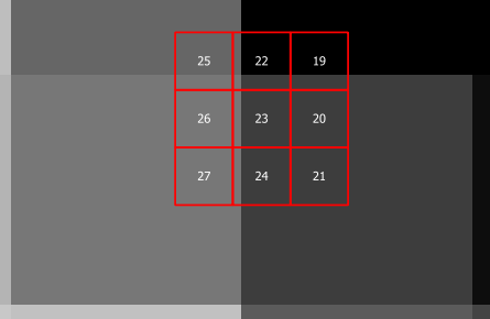
Calculating zonal statistics in R with the extract function in the raster package, I found unexpected behaviour. I have a raster layer of rather large cell size and a polygon layer of relatively small, quadratic polygons. As an example, I want to use these nine polygons 19 - 27 with the raster plotted as background:

enter image description here

extract(raster, polygon, weights=TRUE, normalizeWeights=FALSE)

yields the following result:

[[19]]
          value weight
[1,] -102.39999   0.06
[2,]  -92.79999   0.03

[[20]]
     value weight
 -92.79999   0.06

[[21]]
     value weight
 -92.79999   0.09

[[22]]
          value weight
[1,] -102.39999   0.04
[2,]  -92.79999   0.02

[[23]]
     value weight
 -92.79999   0.04

[[24]]
     value weight
 -92.79999   0.06

[[25]]
     value weight
[1,]   -88   0.06
[2,]   -86   0.03

[[26]]
 value weight
   -86   0.06

[[27]]
 value weight
   -86   0.09

Apparently, the function collects the values of the raster cells overlapping with each polygon and assigns each value a weight corresponding to the area covered by the respective coverage within a polygon. If that worked perfectly, I'd be absolutely satisfied. However, there are some oddities:

  • Why is weight different for polygons 20 and 21, 26 and 27?
  • Why are weights ≠ 1 when a polygon falls completely within a raster cell?
  • Why does polygon 22 only get 2 values instead of 4 (and polygon 23 and 24 1 value each instead of 2)?

The help page states that weights "returns, for each polygon, a matrix with the cell values and the approximate fraction of each cell that is covered by the polygon(rounded to 1/100)". I suppose that weight rather uses a distance measure of the polygon to the raster cell centroid than an actual coverage fraction (?). When using normalizeWeigths=TRUE, this might become irrelevant. However, partly ignoring raster cells that fall within a polygon doesn't seem irrelevant at all.

Does anybody understand why this happens and how to solve this problem?

2
  • As described in the answer here, I could have achieved my goal by doing the analysis using PyQGIS. However, I had reasons to stick to R. So my workaround in the end was the following: I interpolated the input raster (bicubic interpolation) so to obtain a reasonable cell-size. extract then was able to calculate correct mean values for each polygon. However - I'd really like to understand why the function is not able to deal with large raster cell sizes correctly.
    – yenats
    Commented Oct 27, 2017 at 15:09
  • I would highly recommend switching to the exactextractr package for these operations. It returns a precise intersection between the polygon and each given cell and returns the fraction of the cell covered by the polygon. Since it is written in C++ it also has the advantage of being quite a bit faster that raster::extract. You may want to also look at the beta version of terra that just came out, it is intended as a replacement for the raster package and is written in C++ (same developer as raster). Commented Apr 27, 2020 at 22:48

1 Answer 1

1

There are two important points to take into account:

  • extract looks at how much of the cell falls into the polygon, you seem to be asking the opposite question of how much the polygon falls into the cell?

  • the algorithm runs as follow: decompose each cell into 100 cell, look weather each small's cell centroid falls into the polygon

Based on this, we can have tentative answers:

Why is weight different for polygons 20 and 21, 26 and 27?

That's the most tricky one. Are you sure your polygons have the same area? and are projected in an equal area CRS?

Why are weights ≠ 1 when a polygon falls completely within a raster cell?

From above, extract gives you the opposite answer. Seems a little silly, but you could try rasterize the polygon, and vectorise the raster?

Why does polygon 22 only get 2 values instead of 4 (and polygon 23 and 24 1 value each instead of 2)?

Probably the centroid of the small cell (1/100 of the original one) does not fall in the polygon?

You unfortunately did not provide a reproducible example. But here goes a simple check:

library(raster)
library(tidyverse)
library(sf)

r <- raster(nrows=2, ncols=2)
r[] <- 1:4

plot(r)


outer = matrix(c(-2,2,20,2, 20,-20,-2,-20, -2,2),ncol=2, byrow=TRUE)
pts = list(outer)
pl1 = st_polygon(pts)
plot(pl1, add=TRUE)

# as(st_sfc(pl1),"Spatial")

raster::extract(r, as(st_sfc(pl1),"Spatial"), weights=TRUE, normalizeWeights=FALSE)

This gives indeed only one cell! now try to disaggregate first:

    r_disag <- disaggregate(r, 10)

raster::extract(r_disag, as(st_sfc(pl1),"Spatial"), weights=TRUE, normalizeWeights=FALSE, df=TRUE) %>%
  group_by(layer) %>%
  summarise(weight=sum(weight)/10^2)

This shows the four cells! Weird result: the 3 cells have the same area... So try further:

    r_disag <- disaggregate(r, 100)

raster::extract(r_disag, as(st_sfc(pl1),"Spatial"), weights=TRUE, normalizeWeights=FALSE, df=TRUE) %>%
  group_by(layer) %>%
  summarise(weight=sum(weight)/100^2)

Now you get the four cells, with apaprently correct coverage.

This is just to understand how it work... disaggregating by 100 gives you 100^2 more pixels, which will be themselves split into 100 ones... UNfeasible.

Your Answer

By clicking “Post Your Answer”, you agree to our terms of service and acknowledge you have read our privacy policy.

Not the answer you're looking for? Browse other questions tagged or ask your own question.