PostGIS: Interpolate/Cluster geographic points to average points

Question

Setup: PostGIS 3.1, QGIS 3.16

I have a bunch of geographical data (geometries). They show more or less the same route, just measured several times. Due to the many measurements and the GPS precision, the measured points differ, of course:

General visualization of the data:

A more detailed view:

Next to the coordinates the data points keep some additional data, for example the speed of the vehicle which delivered the measurements. This is displayed by the color.

I am interested in the average speed at the track. So I did some interpolation (clustering?) and aggregated the points using PostGIS' ST_SnapToGrid() function:

SELECT
    ST_SnapToGrid(geom, 0.001) as c_geom,
    avg(speed) as avg_speed
FROM my_data
GROUP BY 1

This, naturally, yield a grid-like aggregation:

However, I am searching for a function which I can use like the ST_SnapToGrid() function, but which do not simply trunc the digits of the latitude and longitude but does more like an averaging, so the resulting points are more located on the track itself ("snap to track"). Of course, the speed value needs to be averaged as well.

Desired output:

I am searching for a function which averages lat/lon/speed values within a 10 meters radius or something like that:

I am not even sure if this is possible.

Answer 1

A solution using PostGIS alone.
The Steps are as follows:

1. Generate clusters from the points
2. Get the centre of each point cluster
3. Generate a line that connects each cluster centre point (will also approximate the centreline of the route)
4. Create sampling points at 20m intervals along the line (allowing for 10m radius buffer from each sampling point)
5. Get an average value for 10m buffer around each sampling point.

--1. Create the point clusters
DROP TABLE IF EXISTS points_clustered;
CREATE TABLE points_clustered AS
SELECT geom, st_clusterkmeans(geom, 10) over () AS cluster
FROM points;

--2. Get the centre of each point cluster
DROP TABLE IF EXISTS centers;
CREATE TABLE centers AS
SELECT cluster, ST_Centroid(ST_collect(geom)) AS geom
FROM points_clustered 
GROUP BY cluster;

--3. Get centreline of connecting points
DROP TABLE IF EXISTS clustersline;
CREATE TABLE clustersline AS
SELECT st_makeline(geom) geom FROM 
    (SELECT geom AS geom FROM centers GROUP BY geom ORDER BY st_closestpoint(geom, geom)) AS f;

--4. Create a point on the line every 20 metres **(CHANGE THE EPSG)**
DROP TABLE IF EXISTS clustersline_20m;
CREATE TABLE clustersline_20m AS
WITH line AS 
    (SELECT
        (ST_Dump(geom)).geom AS geom
    FROM clustersline),
linemeasure AS
    (SELECT
        ST_AddMeasure(line.geom, 0, ST_Length(line.geom)) AS linem,
        generate_series(0, ST_Length(line.geom)::int, 20) AS i
    FROM line),
geometries AS (
    SELECT
        i,
        0.0 avg,
        (ST_Dump(ST_GeometryN(ST_LocateAlong(linem, i), 1))).geom AS geom 
    FROM linemeasure)
SELECT
    i,
    avg,
    ST_SetSRID(ST_MakePoint(ST_X(geom), ST_Y(geom)),28355) AS geom
FROM geometries;

--5. Get an average value for 10m buffer of each sampling point.
UPDATE clustersline_20m 
SET avg = subq.avg
FROM 
(
SELECT id, AVG(p.value) avg
FROM points p, clustersline_20m a
WHERE ST_INTERSECTS(ST_BUFFER(a.geom,10), p.geom)
GROUP BY id
) AS subq
WHERE id = subq.id;

Credit to these questions which helped build the answer:
http://blog.cleverelephant.ca/2018/06/polygon-splitting.html
PostGIS or QGIS: Convert unsorted points to a single line by connecting each 2 closest points
How can I transform polylines into points every n metres in PostGIS?

Answer 2

Algorithmic solution

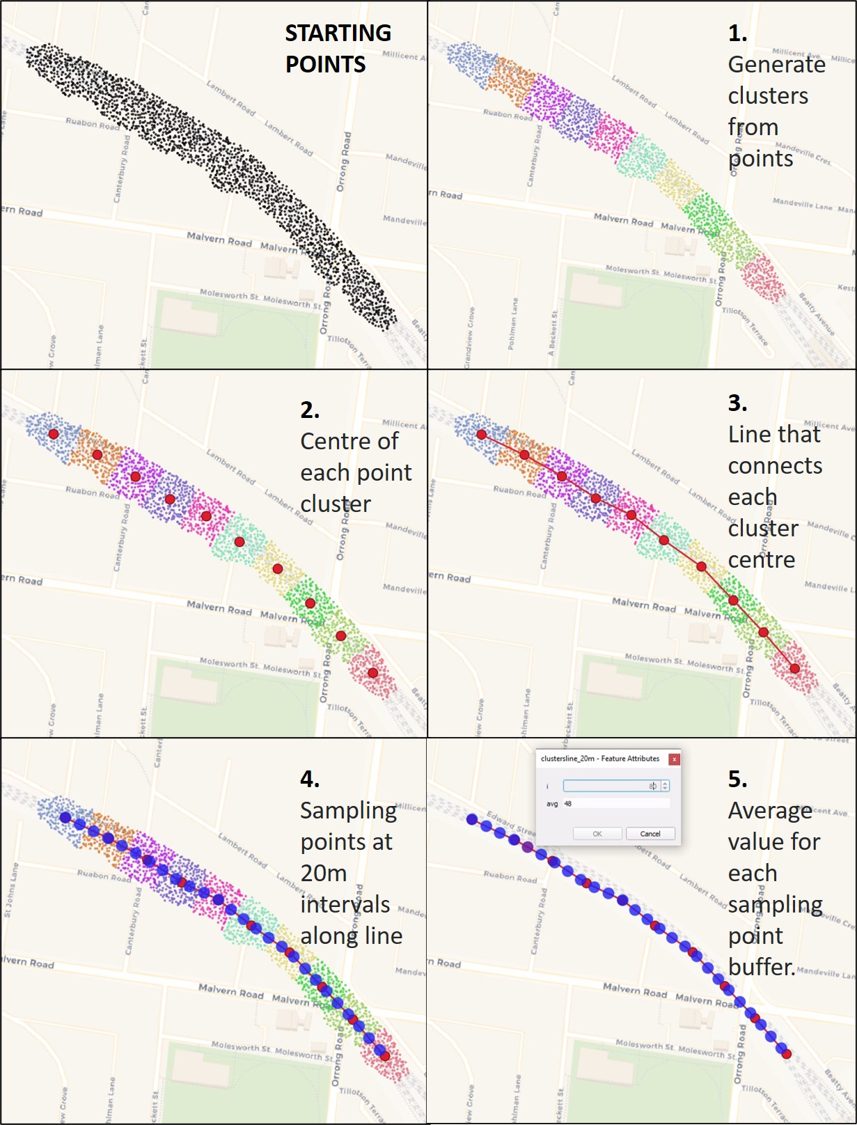
1. Project the points to the line layer
2. Create a new point layer with points at a regular interval along the line
3. For each point of step 2, find the closest point from step 1: this one is the "cluster center" - the point that remains and that gets the mean value of the other points in a certain distance (those that are deleted afterwards).
4. For each cluster center (from step 3), create a buffer and get the mean value for a certain attribute (like speed) of all projected points (from step 1) that fall within the buffer.

Implementation using QGIS:

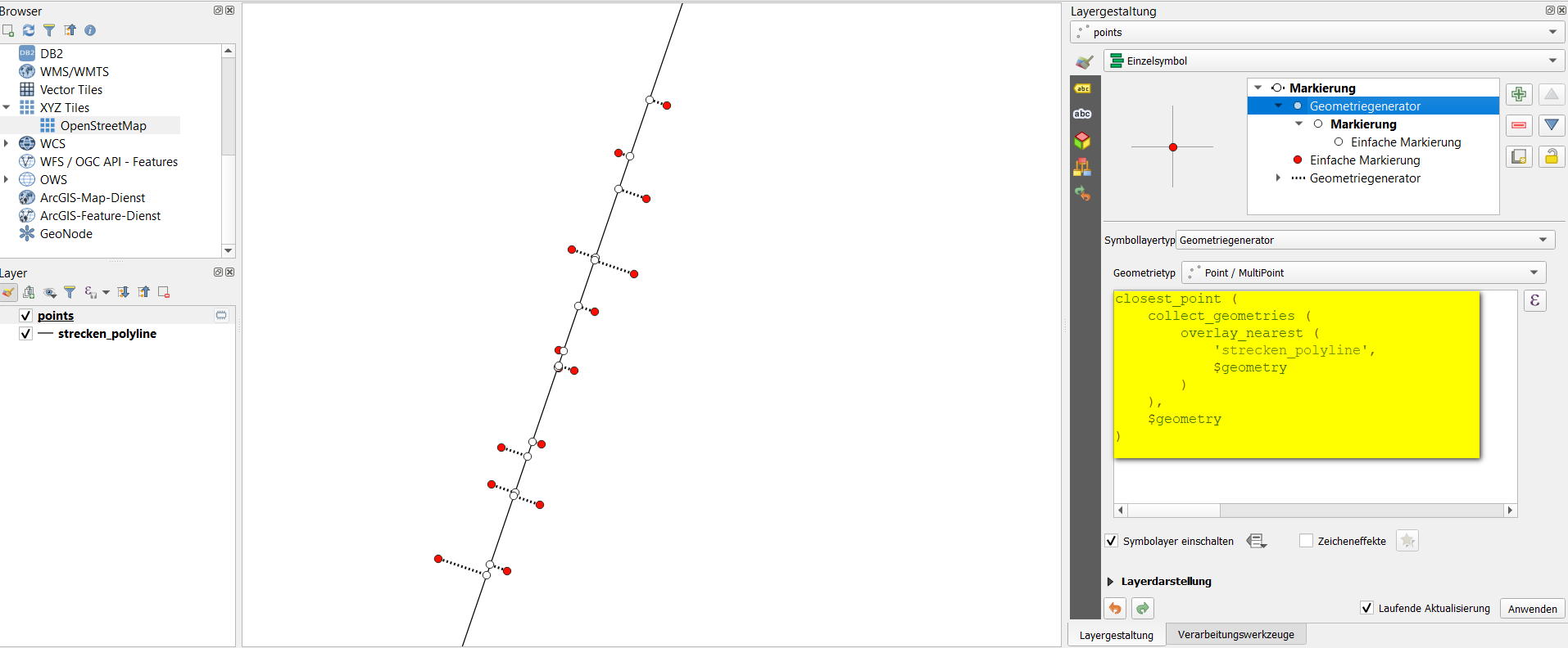
1. Project the points to the line, using an expression like the following on the point layer - us Menu Processing / Toolbox / Geometry by expression to create the points - attributes will be kept:

   closest_point (
       collect_geometries (
           overlay_nearest ( 
               'strecken_polyline', 
               $geometry
           )
       ), 
       $geometry
   )
   

   

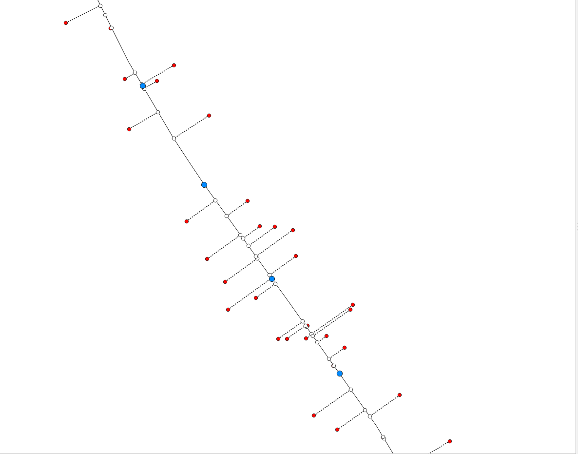
2. Menu Processing / Toolbox / Points along geometry: create regular points along the line - select a distance that fits your date and needs. On the next screenshot, the blue dots are the points created here:

   

3. For each blue dot, find the closest white dot: this will be used as cluster center (thus the points that will be kept and that get the mean value off all other points). This is the expression to use with Menu Processing / Toolbox / Geometry by expression, where projected_points is the name of the point layer created in step 1:

   collect_geometries (
       overlay_nearest( 
           'projected_points', 
           $geometry, 
           limit:=1
       )
   )
   

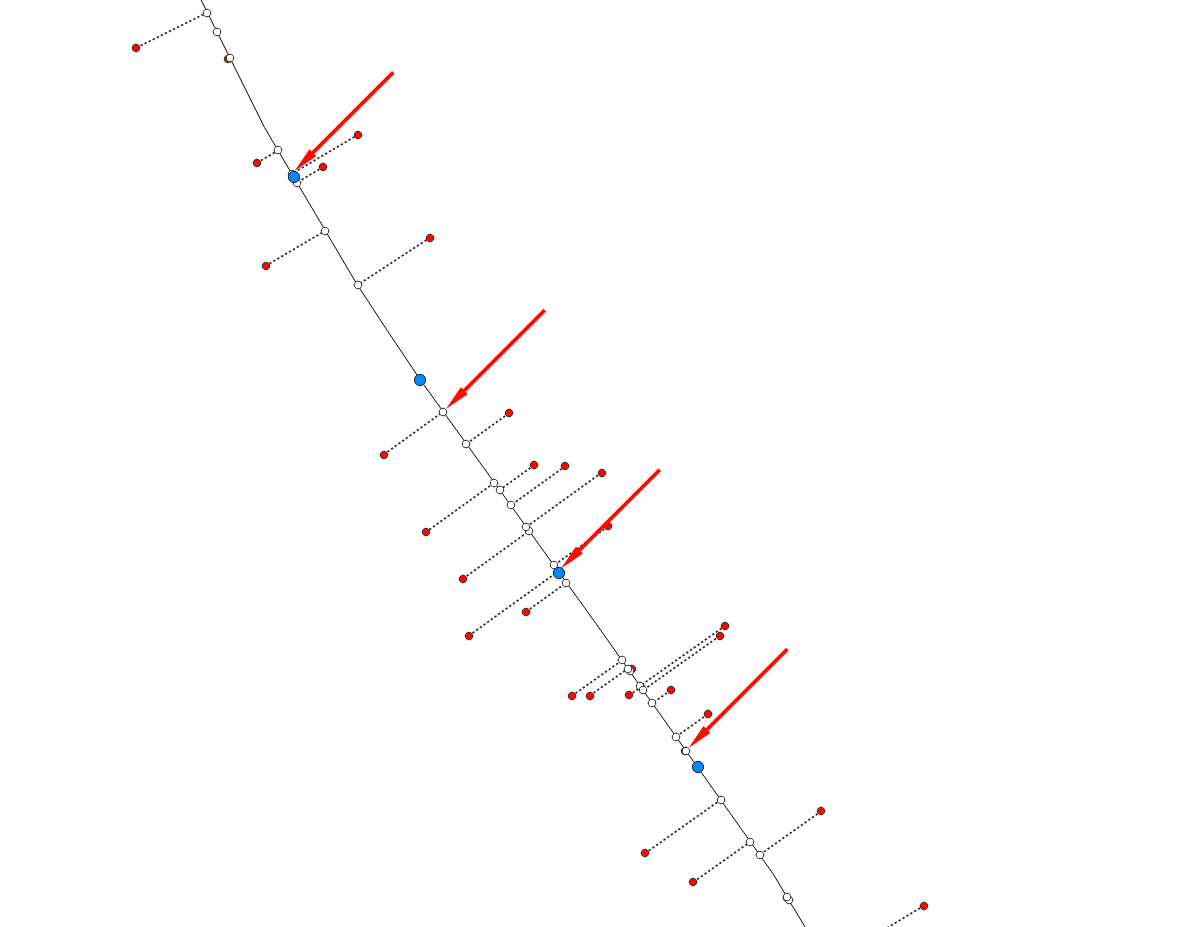
   In the next screenshot, the cluster center is marked by red arows:

   

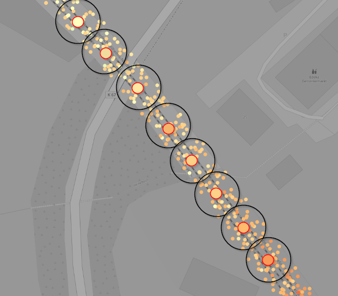
4. Now create a buffer around each cluster center (result from step 3). For the size of the buffer, for demonstration purpose I selected a value of 50 [meters] - use whatever distance fits your data and change the value on line 7 of the following expression. Than, for each point that falls inside this buffer, calculate the mean value for an attribute (here: the field named speed). You can do this by opening the attribute table of the layer with the cluster center (result from step 3) and use the field calculator. Introduce this expression to create a new field with the mean value:

   aggregate( 
       'projected_points', 
       'mean', 
       speed, 
       intersects (
           $geometry, 
           buffer (geometry (@parent), 50)
       )
   )
   

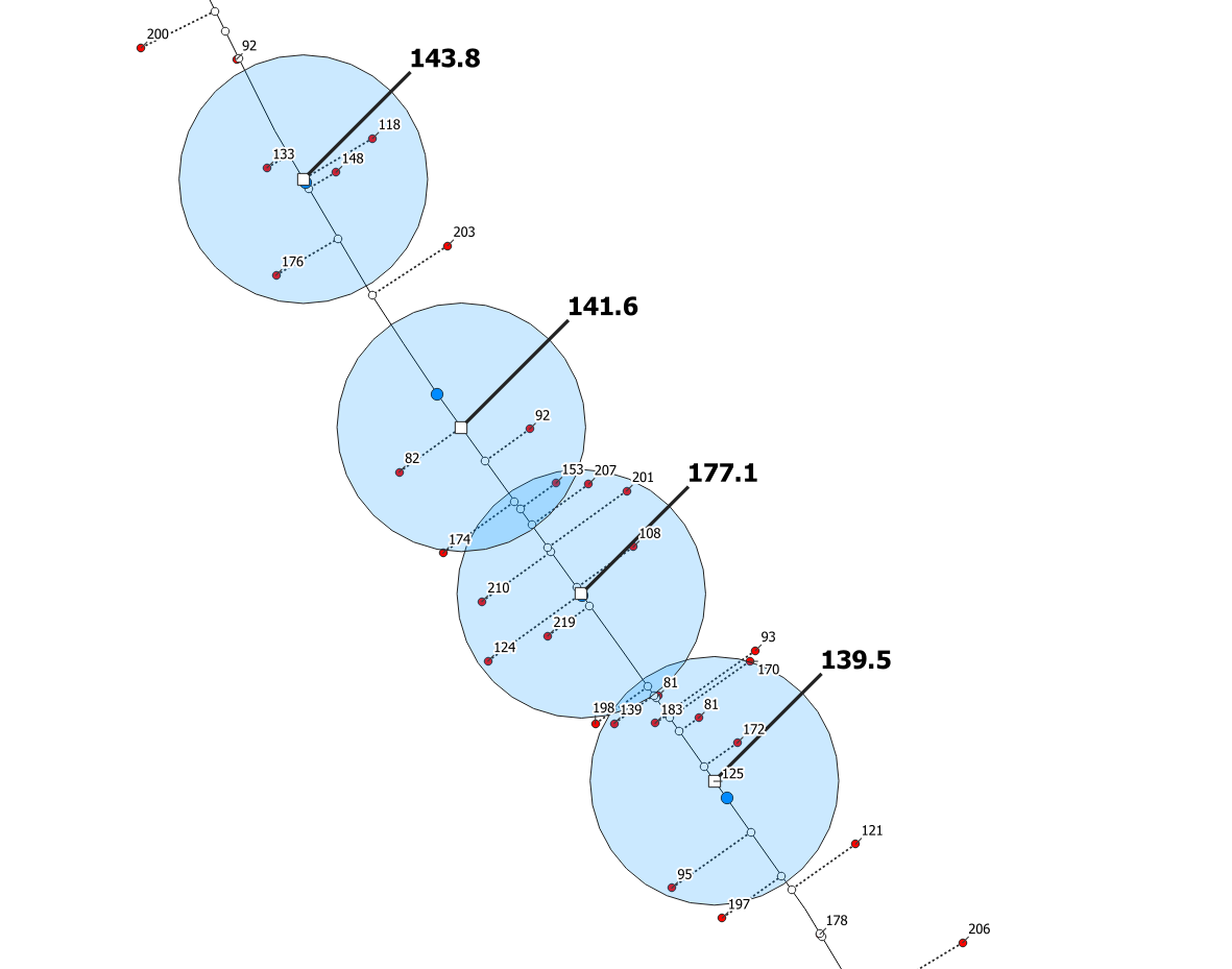
See the result on the next screenshot: the original points (red dots) are reduced to the white squares. Compare the values of the labels that represent the speed field (I used random values from 80 to 220, just to see the effect): the small values nearby the red dots is the speed values in the original data, the bold values is the calculated mean for the points that fall inside the blue buffer (visualized here for better understanding, but it is not necessary to actually create these buffers):

Remarks: as you can see, depending on how far away the nearest projected point (step 1) is from the regular points (step 2), the buffers overlap or have gaps in between - so in some cases not all points are "catched" or some points are "catched" twice. I guess in your data, you have much more points and they are closer together, so this problem should not be too big.

However, there is a possibility to make sure that a) all points are taken into consideration and b) every point is taken into consideration just once. If you would like to do it that way, it's a bit more complicated, but not too much - just leave a comment so that I can add this to the solution.

---

This here is the first variant of the solution - I keep it here as it still might be helpful:

If you have a line-layer (railway, from OpenStreetMap), you can do the following steps. In principle, it works also without an additional line layer, just with the points (simply skip step 1), but than you only have a mean value for each point, based on all point in a certain distance (that you set in the step numbered with 2 below). To create a line from these points would be another question that should be asked separately.

2. Create a buffer around each point with a distance that fits your data.

3. Create a new field on the buffer layer that counts the mean of all values of a particular attribute field of those points that fall inside the buffer. Use this expression (adapted to to filed/layernames you use - I used projected_points for the layer from step 1, and value for an attribute in the original points layer with random values - your field is the one containing the speed information):

    aggregate( 
        'projected_points', 
        'mean', 
        value, 
        intersects (
            $geometry, 
            geometry (@parent)
        )
    )

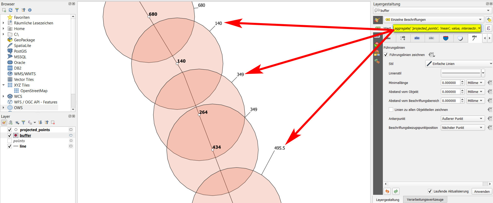
See screenshot, where the expression is used for labeling the buffer:

4. If you want, using a table join, you can join the value calculated in the last step to your original point layer.

Answer 3

Adding a minor detail on Cushen's answer the K-means algorithm can take a max_radius of the clusters as input from version 3.2.0 onwards: postGIS doc

So by passing a parameter of 10 for the max_radius, the number of clusters will increase automatically so that each cluster has a maximin radius of 10m:

st_clusterkmeans(geom, number_of_clusters, max_radius)

(PS I would have added this as a comment, but I do not have enough reputation points)

Answer 4

You actually seems to try to do something called map-matching. I don't know at wich scale do you want to use your algorithm, but if you just group GPS track by cluster or even snap it on the closest road you will face a lot of problems with real life data. GPS data can easily be noisy, especially in urban environnement, where there is a lot of chances to snap on the wrong road, because the network is more dense.

If you goal is to group data which have passed on the same road, either to count, compare vehicles with each other or gather info on the roads, I really encourage you to use map-matching first.

There is a lot of different ways to do this, for exemple:

• Using a paying service: Mapbox, TomTom, Here...
  • Sometimes free for demo
  • Can be costly, and dependant of their map
• Using a free software to install yourself and run with OSM data: GraphHopper, OSRM, ...
  • Free, sometimes there is a demo server too, work with the data you give it (OSM format generally), can run the whole world
  • Needs to be installed and managed, need a big server if you want to run the world efficiently
• Using small scale map-matching tools
  • Qgis plugin: https://github.com/jagodki/Offline-MapMatching
  • Python lib: https://github.com/cyang-kth/fmm

Once your data is properly snapped to your network, it's simpler to cut it like you want, either by using the geometry of your network or by using the snapped points.

Also, this way of trying to cut roads into regular part is also a complicated problem (intersections, map changing over time, ...) and is usually linked to the idea of trying to find concentration of something along the road (event, speed, ...). Your can find more info on this subject for exemple by looking here (where they introduce the notion of lixel - linear pixel): https://www.sciencedirect.com/science/article/pii/S0198971508000318