How to cluster 1000+ points into 50 clusters based on geospatial proximity in R?

Question

Sample data:

set.seed(123)
lon <- runif(1200, 72.6, 73.2)
lat <- runif(1200, 18.8, 19.6)

df <- data.frame(lon, lat)

Progress so far:

geo.dist = function(df) {
  require(geosphere)
  d <- function(i,z){         # z[1:2] contain long, lat
    dist <- rep(0,nrow(z))
    dist[i:nrow(z)] <- distHaversine(z[i:nrow(z),1:2],z[i,1:2])
    return(dist)
  }
  dm <- do.call(cbind,lapply(1:nrow(df),d,df))
  return(as.dist(dm))
}

hc <- hclust(geo.dist(df))
clust <- cutree(hc, k=50)

#Visualise the results

ggplot()+
  geom_point(data=df,aes(x=lon, y=lat, col=as.factor(clust)))+
  theme(legend.position = 'none')

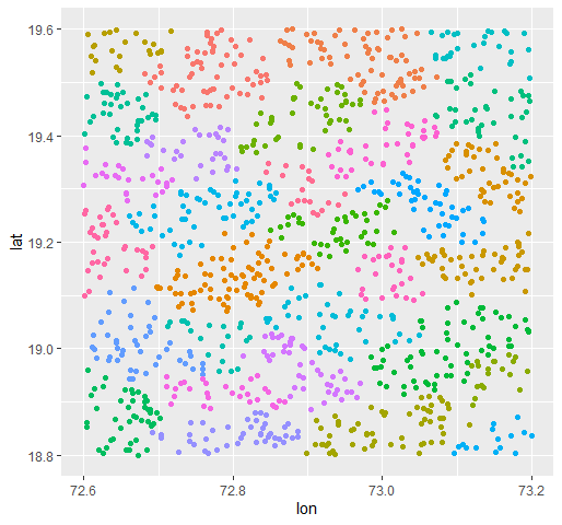
As visualized from the plot, the results are very inconsistent. (The sample data is giving a bit better still, as the points are scattered well) Is there any way I can cluster them? Without using Hierarchical or K-Means?

Found one similar approach here: https://www.supplychaindataanalytics.com/proximity-based-spatial-customer-grouping-in-r/

But it is providing NA for me. Don't know why.

Any help would mean a lot!

Answer 1

You are applying an ecological fallacy in the interpretation of something that you found online in relation to your data and expected outcome. One must consider realistic expectations, method and fit. An optimal cluster solution of a continuous random field may not be one that is visually validated.

Just because you define n as 50 does not mean that 50 clusters are actually supported. Often, when using something like k-means, you evaluate a range of cluster solutions and then select one with the best fit using a metric such as the silhouette. Here is your intended implementation using hierarchical clustering.

library(ggplot2)
library(sp)

set.seed(123)
d <- data.frame(lon=runif(1200, 72.6, 73.2), 
                lat=runif(1200, 18.8, 19.6))

dm <- sp::spDists(as.matrix(d), longlat = TRUE)

hc <- stats::hclust(dist(dm))
  clust <- stats::cutree(hc, k=50)

ggplot()+
  geom_point(data=d,aes(x=lon, y=lat, col=as.factor(clust)))+
    theme(legend.position = 'none')

However, I would go with a threshold value and not a specific k. A solution using d(h) = 500, which is close to the 1st quartile of scaled distances, results in k = 30. If I define d(h) = 350 the cluster solution results in a k = 55. In this way you side-step optimal cluster solutions, with hard a bounded k, and base the outcome on a distance criteria.

clust <- stats::cutree(hc, h=500)
  ggplot()+
    geom_point(data=d,aes(x=lon, y=lat, col=as.factor(clust)))+
      theme(legend.position = 'none')

summary(as.vector(dist(dm)))
  length(unique(clust))

I provided a similar answer here but, project into a distance based projection to have an explicit distance threshold and cluster on the coordinates rather than a distance matrix.