Extent not found on NASA's Black Marble monthly images - How to set it?

Question

I downloaded NASA's Black Marble monthly nighttime light (NTL), VNP46A3. The product is in .h5 format and it contains the radiance NTL raster as well as the scientific data sets (SDS) in order to remove bad quality pixels etc.

When I import the .h5 raster I am getting this warning: Warning message: [sds] unknown extent.

Then I converted the .h5 into a SpatRaster using the below code:

library(terra)
s <- sds(paste0(wd, "VNP46A3.A2018182.h06v05.001.2021125183820.h5"))

# extract single image as spatraster from h5
r <- s[5] # I extract the radiance raster

writeRaster(r, paste0(wd, "rad.tif"))

When I type ext(r), I get:

class       : SpatRaster 
dimensions  : 2400, 2400, 1  (nrow, ncol, nlyr)
resolution  : 1, 1  (x, y)
extent      : 0, 2400, 0, 2400  (xmin, xmax, ymin, ymax)
coord. ref. :  
source      : r.tif 
name        : AllAngle_Composite_Snow_Free 
min value   :                            0 
max value   :                        65535 

My question is how can I set the correct extent (and CRS) to the r raster in R?

I am using R 4.3.1 and RStudio RStudio 2023.06.2+561.

Answer 1

Read the data using terra::rast - I'm not sure what sds wins you here, this works:

r <- rast("VNP46A3.A2018182.h06v05.001.2021125183820.h5")

Define the coordinates to be lat-long WGS84:

crs(r) = "epsg:4326"

Now the documentation says the data are 15 arc-minute cells. That means for these 2400x2400 grids they span:

> 2400*(15/(60*60))
[1] 10

exactly ten by ten degrees.

Which ten degrees? That's encoded in the file name. Set these up:

h = 6
v = 5

Then you can reset the extent by computing the appropriate offsets and adding ten degrees:

ext(r) = c(-180+h*10,-180+(h+1)*10, (8-v)*10,(8-v+1)*10)

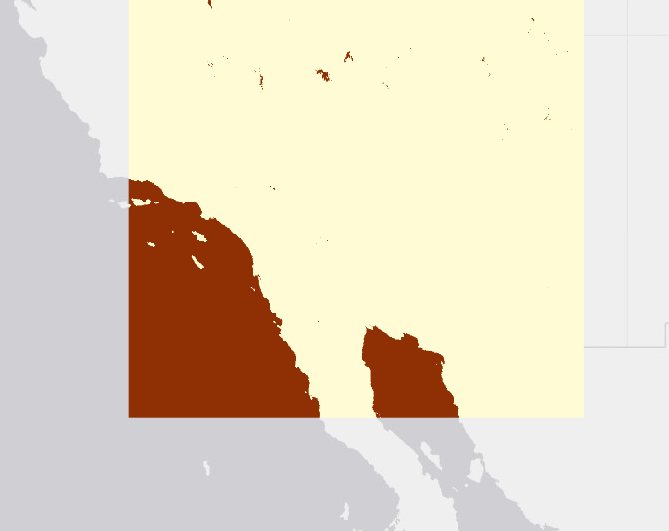
And we can plot on a map background to confirm:

tm_shape(r[[1]]) + tm_raster()

Which looks good. There's some assumptions here, like the WGS84 coordinate system and the grid being aligned to WGS84 10 degree grids, but this seems to work. Its possible it should be shifted by half a cell size. Check it out on a few more files.

If you want to get the tile numbers from the data, they are stored as netcdf global attributes, which you can get from the file using the ncdf4 package:

> library(ncdf4)
> n = nc_open("VNP46A3.A2018182.h06v05.001.2021125183820.h5")
> as.numeric(ncatt_get(n, 0)$VerticalTileNumber)
[1] 5
> as.numeric(ncatt_get(n, 0)$HorizontalTileNumber)
[1] 6
> nc_close(n) #tidyup

Now let's put this all in a function:

readA3 <- function(f){

    r = terra::rast(f)
    crs(r) = "epsg:4326"
    n = ncdf4::nc_open(f)
    v = as.numeric(ncdf4::ncatt_get(n, 0)$VerticalTileNumber)
    h = as.numeric(ncdf4::ncatt_get(n, 0)$HorizontalTileNumber)
    ncdf4::nc_close(n)

    ext(r) = c(-180+h*10,-180+(h+1)*10, (8-v)*10,(8-v+1)*10)
    r
    
}

Which we can use like this:

 h6v6 = readA3("./VNP46A3/2018/182/VNP46A3.A2018182.h06v06.001.2021125183917.h5")
 h7v6 = readA3("./VNP46A3/2018/182/VNP46A3.A2018182.h07v06.001.2021125183820.h5")
 h6v5 = readA3("./VNP46A3/2018/182/VNP46A3.A2018182.h06v05.001.2021125183820.h5")

using the bulk-downloaded files and folders from the "Data Archive". Plotting shows they are in the right place, but beware that tmap seems to do a bit of approximation (or possibly transform to web mercator) which can show gaps - saving as TIF and loading into QGIS shows two tiles meeting at a perfect corner which is telling me this is most likely spot on:

As noted elsewhere, its possible modern versions of GDAL can interpret the metadata and work this out for themselves, but my installation with GDAL 3.4.1 doesn't.

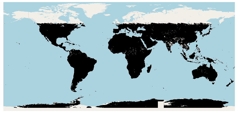
As a final test I downloaded all the images from one folder, looped over them, converted every one's first layer to a TIF, and loaded all 300 or so layers into QGIS.