Polygon and raster in the same plot do not align

Question

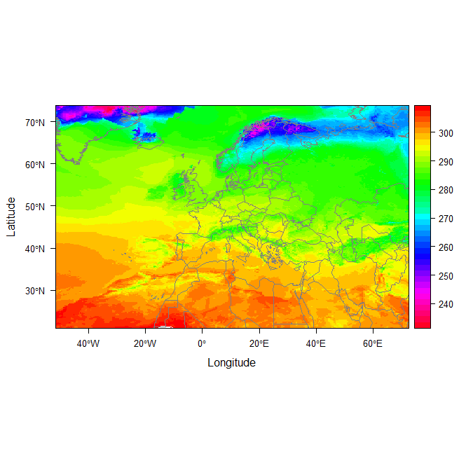
I can't manage to plot a raster and boundary of country (sp data frame) in the same plot. The data (lon,lat,value) are in mat data frame. The grid is not regular and comes from a climate change ncdf file.

Here is the ncdump original file :

7 variables (excluding dimension variables):
        double lat[rlon,rlat]   
            bounds: lat_vertices
            long_name: latitude coordinate
            standard_name: latitude
            units: degrees_north
        double lat_vertices[vertices,rlon,rlat]   
            units: degrees_north
        double lon[rlon,rlat]   
            bounds: lon_vertices
            long_name: longitude coordinate
            standard_name: longitude
            units: degrees_east
        double lon_vertices[vertices,rlon,rlat]   
            units: degrees_east
        double time_bnds[bnds,time]   
        float hfss[rlon,rlat,time]   
            standard_name: surface_upward_sensible_heat_flux
            long_name: Surface Upward Sensible Heat Flux
            units: W m-2
            original_name: HFX
            cell_methods: time: mean
            missing_value: 1.00000002004088e+20
            _FillValue: 1.00000002004088e+20

            grid_mapping: rotated_latitude_longitude
            coordinates: lat lon
            positive: up
        int rotated_pole[]   
            grid_mapping_name: rotated_latitude_longitude
            grid_north_pole_latitude: 39.25
            grid_north_pole_longitude: -162

I try to plot this grid with raster and levelplot package.

library(raster)
library(rasterVis)
library(rworldmap)

data(wrld_simpl)
colnames(mat) <-c("lon","lat","value")

x.min=min(mat$lon)
x.max=max(mat$lon)
y.min=min(mat$lat)
y.max=max(mat$lat)

v.min=min(mat$value)
v.max=max(mat$value)

breaks=seq(v.min,v.max,2)
colour=rev(rainbow(length(breaks), alpha=1))

ras <- raster(nrows=453, ncols=453,xmn=x.min,xmx=x.max, ymn=y.min, ymx=y.max)
rvm <- matrix(mat[,3],453,453,byrow=TRUE)
ras[]=rvm[nrow(rvm):1,]

levelplot

levelplot(ras,at=breaks,col.regions=colour, margin = FALSE) +
layer(sp.polygons(wrld_simpl, fill = NA, col = "grey50"))

and plot

Of course, SP polygon (in WGS84) does not fit to the original ncdf grid. The original data frame is available here :

[https://drive.google.com/file/d/0Byd6YJGGADrfN255ZGhhTjRSUkU/view?usp=sharing][2]

Answer 1

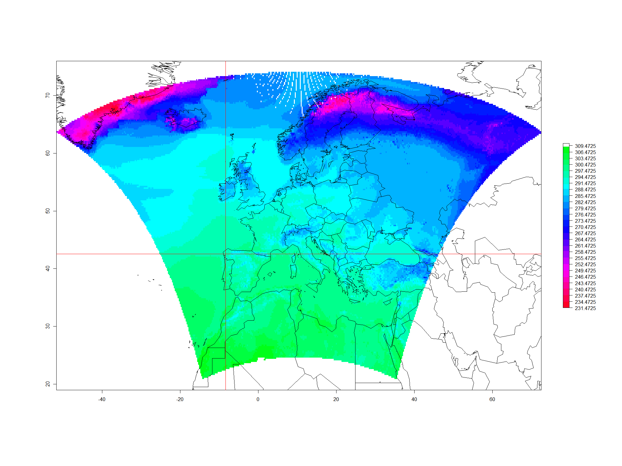
The problem here is that, when you redefined the extension of the raster, the real coords of the data changed. You can see that raster values are wrong located if you show some guidelines (I've used Santiago de Compostela coords). Here process:

1. Tryout with you data and using base R plotting system.
2. Tryout defining the same exact CRS for the raster and wrld_simpl. (not working)
3. Tryout defining a new CRS for the raster for general EU views. (not working)
4. Tryout avoiding the raster definition within your code and using the function rasterFromXYZ() instead. --> WORKED

Here is the code:

library(raster);    library(rasterVis);    library(rworldmap)
library(maptools);    library(raster);    library(lattice);
library(gdal);    library(plotly)

load("mat.rda");    data(wrld_simpl);    colnames(mat) <-c("lon","lat","value")
x.min=min(mat$lon);    x.max=max(mat$lon)
y.min=min(mat$lat);    y.max=max(mat$lat)
v.min=min(mat$value);    v.max=max(mat$value)
breaks=seq(v.min,v.max,2)
colour=rev(rainbow(length(breaks), alpha=1))
ras <- raster(nrows=453, ncols=453,xmn=x.min,xmx=x.max, ymn=y.min, ymx=y.max)
rvm <- matrix(mat[,3],453,453,byrow=TRUE)
ras[]=rvm[nrow(rvm):1,]

# 1. Plot them, one layer after another
plot(ras)
plot(wrld_simpl, add=TRUE)

# 2. Plot them with the same exact CRS
crs(ras) <- crs(wrld_simpl)
plot(ras)
plot(wrld_simpl, add=TRUE)
abline(h = 42.883, v = -8.533, col="red") #location of Santiago de Compostela

# 3. CRS to one of the common EPSG used for EU view:
crs(ras) <- CRS("+init=epsg:3035")
plot(ras)
plot(wrld_simpl, add=TRUE)
abline(h = 42.883, v = -8.533, col="red") #location of Santiago de Compostela

# 4. represent your xyz data directly like here:
ras2 <- rasterFromXYZ(mat, res = 0.25, crs = crs(wrld_simpl), digits = 0)
plot(ras2, breaks = breaks, col = colour)
plot(wrld_simpl, add=TRUE)
abline(h = 42.883, v = -8.533, col="red") #location of Santiago de Compostela

Here is the final plot: