Comparison with different resolution rasters

Question

The purpose is to compare the fractional snow cover of the coarser pixel to the binary snow cover (0 for no-snow and 1 for snow) of lower resolution pixels. Both the datasets are of the same area and share the same WGS84 coordinates. Below are two of the methods that I am thinking of:

As I understand random point sampling is independent of resolution in ArcGIS. So, I have two rasters one with coarser resolution say in kilometers and the other one is of finer resolution in meters. I create random points for each of the rasters. Then I run the "Extract multi values to point" tool to extract the pixel values of the attributes to these points. Please note that the attributes has to do with fractional area coverage in percentage (0-100%) in a pixel for one of the rasters, whereas the other raster which is of 500m resolution has binary/discrete values i.e. 0 /1 . The goal is to do a comparison between the point values based on fractional area coverage/percentage of each cell in the coarser raster to the binary data finer resolution raster. So for example on a given day, the fractional covered area is 96% for a particular coarser pixel. As I know the coarser pixel has approximately 165 pixels, and so for that given day 60 of the finer resolution pixels have value 1. Hence, I add them and divide it by 165, basically ((60/165)*100)= 36.36%. I can then compare the two fractional area values i.e. 96% with 36.36%

So far I have found that there are 165 points representing the smaller pixels that lie in a single coarser cell. My question is somewhat similar to this question with the only difference that temporal resolution is same.

Will this be a valid comparison between the two sets of random point sampling, even though the resolution of the rasters is quite different?

Second Approach

I find the number of pixels in the coarser pixel, which is approximately 165, and then for those 165 pixels I add the binary one values of these pixels and divide them by total number of pixels which is 165, this might give me fractional area coverage of snow. I can then compare the fractional area coverage of the coarser pixel with the fractional area coverage of the 165 pixels. But even in this case, I am noticing that some of the pixels lie right on the boundary line of the coarser pixel.

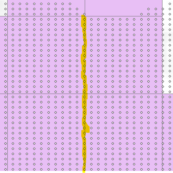
The whole purpose is to comparison in such a way that one resampling of resolution can be avoided.

Answer 1

I am not clear exactly what you are wanting to test here. Do you have a hypothesis? You can certainly take a sampling approach in evaluating the "accuracy" of the lower resolution binominal classification along with hypothesis testing the distributional equivalence of the binominal classes.

Here is a worked example, in R, of what testing a hypothesis and evaluating accuracy would look like. The example is provided in R because ArcGIS just does not have the tools to perform this type of analysis.

First, let's add our required libraries and create some example data. Please note that the higher resolution raster contains random values on a proportional scale and the lower resolution data is binominal thus, emulating your problem. The results in the example cannot be interpreted literally due to the binominal data being a thresholded function of the higher resolution proportional data but, it gives the analytical framework for real data.

library(raster)
library(sp)
library(exactextractr)
library(rfUtilities)

r.high <- raster(nrows=180, ncols=360, xmn=571823.6, xmx=616763.6, ymn=4423540, 
            ymx=4453690, resolution=100, crs = CRS("+proj=utm +zone=12 +datum=NAD83 
            +units=m +no_defs +ellps=GRS80 +towgs84=0,0,0"))
    r.high[] <- runif(ncell(r.high),0,1)
r.low <- aggregate(r.high, fact=6, fun=median)
  r.low <- reclassify(r.low, matrix(c(0,0.5,0,0.5001,1,1), 
                      ncol=3, byrow=TRUE))

par(mfrow=c(1,2))
  plot(r.high)
  plot(r.low)

Now that we have a reproducible example we can create a random sample, across the higher resolution raster (which will contain the associated cell values) and then extract the values for the low-resolution data.

rs <- sampleRandom(r.high, 5000, sp=TRUE)
  rs@data <- data.frame(rs@data, extract(r.low, rs))
    names(rs) <- c("high_res", "low_res")

For hypothesis testing, using the Kruskal-Wallis Test, we can decide whether the population distributions are identical without assuming a normal distribution. The null hypothesis is that the snow proportions in the higher resolution data are identical populations across the binominal [0,1] values.

kruskal.test(rs$high_res ~ rs$low_res, data = rs) 

We can also use the log loss statistic to evaluate the accuracy, of the low-resolution data, based on penalizing the magnitude of the "miss-classification". Make sure that, if you are dealing with percentages, that you rescale to a 0-1.

logLoss(y=rs$low_res, p=rs$high_res)

We can also evaluate the data by splitting out the two classes. The Kolmogorov-Smirnov test evaluates the distributional equivalence and Mann-Whitney is a nonparametric test where the null hypothesis is that for randomly selected values x and y from two populations, the probability of x being greater than y is equal to the probability of y being greater than x.

ks.test(rs@data$high_res[which(rs$low_res == 1)], 
        rs@data$high_res[which(rs$low_res == 0)])
wilcox.test(rs@data$high_res[which(rs$low_res == 1)], 
            rs@data$high_res[which(rs$low_res == 0)], 
            alternative = "g")

Alternately you can just intersect the data by coercing the lower resolution data to polygons and extracting the values from the higher resolution data. You can then summarize the values or relate the data into a dataset and calculate an evaluation statistic.

Here, we coerce to polygons and extract high-resolution raster values to low-resolution polygons (pixels)

r.low <- rasterToPolygons(r.low, dissolve=FALSE)
  v <- exact_extract(r.high, as(r.low, "sf"))

Now, simply calculate a few statistical moments

v.stats <- lapply(v, function(x) summary(x[,1]))
  head( v.stats <- as.data.frame(do.call(rbind, v.stats)) )

Or, we can also relate values and calculate log loss

v.df <- do.call(rbind, v)
 v.df <- data.frame(v.df, r.low$layer)
    v.df <- data.frame(ID=unlist(lapply(strsplit(rownames(v.df), "[.]"), 
                        function(x) x[1])), v.df)   

r.low@data <- data.frame(ID=1:nrow(r.low), r.low@data) 
  names(r.low) <- c("ID", "snow_class")
  
v.df <- merge(v.df,r.low@data, by="ID", all = TRUE)   
  names(v.df) <- c("ID", "snow.pct", "pixel_fraction", "snow_class")
 
logLoss(v.df[,"snow_class"], v.df[,"snow.pct"])

To account for potential misalignment issues you can filter the resulting extracted data by the "coverage_fraction" column, or as I later change it to "pixel_fraction". This is the fraction of the intersection of each given pixel and the polygon. So, a 0.2 would be a 20% overlap in the intersection. You can choose a threshold and remove any pixel value that does not adhere to the fractional overlap.