You can't modify the coordinates by hand like that easily without messing-up your LAS object. LAS objects are designed to be as close as possible to the las specification which imply that it is hard to touch a LAS object without understanding the specifications.
First you need to understand that numbers are stored in a LAS file as integers using a scale factor and an offset. Basically the scale factor is the accuracy of the positioning. 0.01 means a centimetre accuracy, 0.001 is millimetre (or 0.001 feet if coordinates are in feet). I already wrote a comprehensive answer on this topic.
That being said, let do some math. Let say you have a point cloud 1000 x 1000 m with an accuracy of 0.01 i.e. centimetre accuracy (do the math with your own numbers). You want to shrink that in [0,1] so you want to scale your point-cloud to 1/1000th. With an accuracy of 0.01 your points will no longer be distinct. For example a point at X = 12345.12 m will be at e.g. X = 0.25 and a point 10 m farther at X = 12355.00 m will also be at X = 0.25. You need to change your accuracy if you want to write that in a LAS file. With an accuracy of 0.00001 the previous example may become X = 0.25123 and X = 0.25134 so the two points are now distinct.
If your point-cloud has an accuracy of 0.01 and you want to shrink to 1/1000th preserving the same relative accuracy you need an accuracy of 0.01/1000 = 0.00001.
So first you must start by doing the math for your point cloud and modify the header of the LAS object consequently. Here I'm using a 250 x 250 point-cloud with a scale factor of 0.01 on XYZ. To preserve the accuracy I need a scale factor of 0.01/250 = 4/100000. So, 10-5 is ok. For Z 10-4 is enough but we can use 10-5 to be consistent.
library(lidR)
LASfile <- system.file("extdata", "Megaplot.laz", package="lidR")
las = readLAS(LASfile)

las@header@PHB[["X scale factor"]] <- 1e-5
las@header@PHB[["Y scale factor"]] <- 1e-5
las@header@PHB[["Z scale factor"]] <- 1e-5
las@header@PHB[["X offset"]] <- 0
las@header@PHB[["Y offset"]] <- 0
las@header@PHB[["Z offset"]] <- 0
Then I retrieve the bounding box. You can also use min(las$X) and so on if you want.
xmin <- las@header@PHB[["Min X"]]
ymin <- las@header@PHB[["Min Y"]]
zmin <- las@header@PHB[["Min Z"]]
xmax <- las@header@PHB[["Max X"]]
ymax <- las@header@PHB[["Max Y"]]
zmax <- las@header@PHB[["Max Z"]]
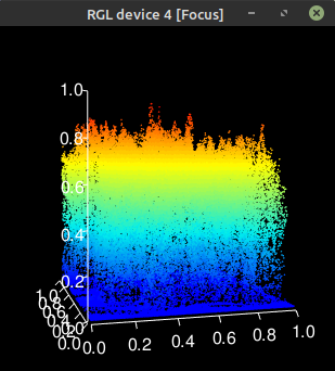
Then I scale the point cloud. Pretty much like you did but you must avoid using las@data$X and use las$X instead. Using las@data$ you are accessing the data directly. With las$ your are using the $ operator defined for LAS objects. And this operator is overloaded so it validates and fixes the input to be compliant with the LAS specification and updates automatically what must be updated. In short it ensures your object is valid with respect to the information in the header (we updated the header to fit our need) and warns you otherwise. See also ?las_utilities.
las$X <- (las$X - xmin)/(xmax - xmin)
las$Y <- (las$Y - ymin)/(ymax - ymin)
las$Z <- (las$Z - zmin)/(zmax - zmin)
Lastly I clear the CRS both erasing the proj4string and cleaning the header.
projection(las) <- CRS()
las@header@VLR <- list()
Now we can check if everything is good.
las
#> class        : LAS (v1.2 format 1)
#> memory       : 6.2 Mb
#> extent       : 0, 1, 0, 1 (xmin, xmax, ymin, ymax)
#> coord. ref.  : NA
#> area         : 0.9996136 units²
#> points       : 81.6 thousand points
#> density      : 81621.54 points/units²
las_check(las)
#>
#>  Checking the data
#>   - Checking coordinates... ✓
#>   - Checking coordinates type... ✓
#>   - Checking coordinates range... ✓
#>   - Checking coordinates quantization... ✓
#>   - Checking attributes type... ✓
#>   - Checking ReturnNumber validity... ✓
#>   - Checking NumberOfReturns validity... ✓
#>   - Checking ReturnNumber vs. NumberOfReturns... ✓
#>   - Checking RGB validity... ✓
#>   - Checking absence of NAs... ✓
#>   - Checking duplicated points... ✓
#>   - Checking degenerated ground points... ✓
#>   - Checking attribute population...
#>    ⚠ 'PointSourceID' attribute is not populated.
#>    ⚠ 'EdgeOfFlightline' attribute is not populated.
#>   - Checking gpstime incoherances ✓
#>   - Checking flag attributes... ✓
#>   - Checking user data attribute... ✓
#>  Checking the header
#>   - Checking header completeness... ✓
#>   - Checking scale factor validity... ✓
#>   - Checking point data format ID validity... ✓
#>   - Checking extra bytes attributes validity... ✓
#>   - Checking the bounding box validity... ✓
#>   - Checking coordinate reference sytem... ✓
#>  Checking header vs data adequacy
#>   - Checking attributes vs. point format... ✓
#>   - Checking header bbox vs. actual content... ✓
#>   - Checking header number of points vs. actual content... ✓
#>   - Checking header return number vs. actual content... ✓
#>  Checking preprocessing already done
#>   - Checking ground classification... yes
#>   - Checking normalization... yes
#>   - Checking negative outliers... ✓
#>   - Checking flightline classification... no
extent(las)
#> class      : Extent
#> xmin       : 0
#> xmax       : 1
#> ymin       : 0
#> ymax       : 1
plot(las, axis = T, clear_artifacts = F)


