How to produce a gridded map in R where each grid cell represents the sum of points occurring in the grid?

Question

I want to produce a gridded map where each grid cell represents the sum of points falling within the grid using R. I have seen similar questions for R here, here, and here for Phyton. But could not get what I needed from none of them.

I have got the gridded map plotted onto a shapefile of the Neotropical region from here https://figshare.com/articles/dataset/Neotropical_region_a_shapefile_of_Morrone_s_2014_biogeographical_regionalisation/3569361 and the distribution of species on the map (each point represents an individual of each species in a specific geographic location). The distribution of points was downloaded from GBIF using the gbif R function from the dismo R package.

To get what I need, these points should be summarised by species per cell so that I get the number of species (irrespective of the number of individuals) that fall within each grid cell. Thus, I can plot the gridded map over the shapefile, coloured by the number of species.

I am a newbie to spatial analysis and have sparse knowledge about doing this in R. So my apologies if it is a very simple question. Any hint is very welcome!

Here is the code I used to get what I have so far:

# Load required packages
library(rgdal)
library(raster)
library(rgeos)
library(dismo)


#retrieve occurrences of Allagoptera species from GBIF
alag <- gbif("Allagoptera", "*", geo=TRUE)

#filter those with latitude and longitude data
alagl <- subset(alag, !is.na(lon) & !is.na(lat))

#I followed the tutorial in the RFunctions blog to create the grids:
#https://rfunctions.blogspot.com/2014/12/how-to-create-grid-and-intersect-it.html
#I just replaced the shapefile with the one for the Neotropics and modified the comments accordingly. 

# Load the Neotropical shapefile.
#Data come from here:
#https://figshare.com/articles/dataset/Neotropical_region_a_shapefile_of_Morrone_s_2014_biogeographical_regionalisation/3569361

#Function 'download.shapefile' comes from here: 
#https://www.r-bloggers.com/2013/09/an-r-function-to-download-shapefiles/

download.shapefile("https://figshare.com/articles/dataset/Neotropical_region_a_shapefile_of_Morrone_s_2014_biogeographical_regionalisation/3569361?file=5646714",
                          "Lowenberg_Neto_2014")

neo <- readOGR(choose.files(), "Lowenberg_Neto_2014") 


# Plot the shape to see if everything is fine.
plot(neo)

# Create an empty raster.
grid <- raster(extent(neo))

# Choose its resolution. I will use 1 degree of latitude and longitude. (It was originally 2).
res(grid) <- 1

# Make the grid have the same coordinate reference system (CRS) as the shapefile.
proj4string(grid)<-proj4string(neo)

# Transform this raster into a polygon to get a grid, but without the shapefile.
gridpolygon <- rasterToPolygons(grid)

# Intersect the grid with the Neotropical shapefile. 
neo.grid <- intersect(neo, gridpolygon)

# Plot the intersected shape to see if everything is fine.
plot(neo.grid)

# add the points corresponding to species occurrences
points(alagl$lon, alagl$lat, col='orange', pch=20, cex=0.75)
# plot points again to add a border for better visibility
points(alagl$lon, alagl$lat, col='red', cex=0.75)

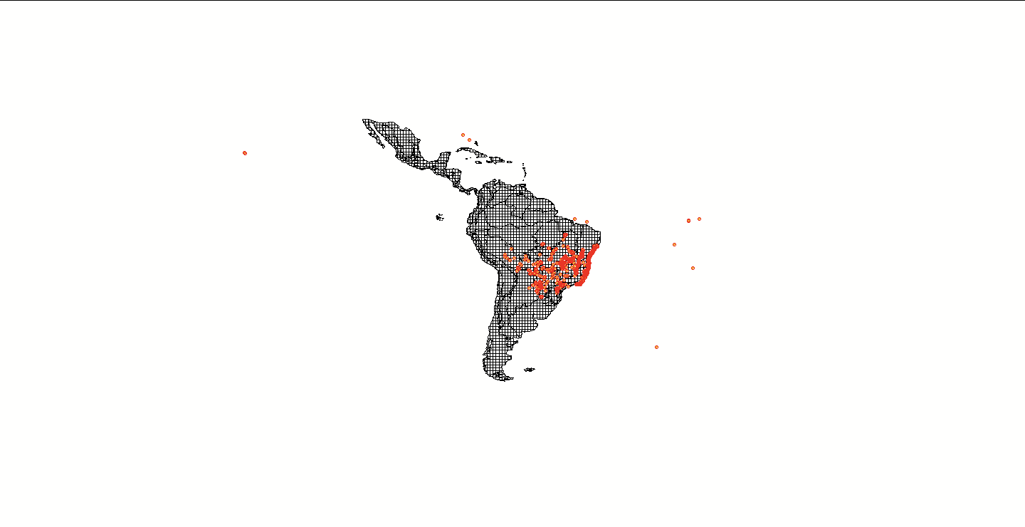
Here is the map I got:

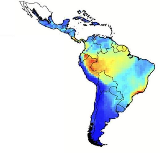
And here is an example of map I am looking for (source: DOI: 10.1371/journal.pone.0152468):

Answer 1

Here's the approach I would take. The general idea is that we create a grid over your countries, then we do a spatial join to the grid then count the number of observations in each grid.

In this example, I just count the number of points. This does not at all match what you provided as an example image. There may be a field that has a population count that should be used as a weight.

library(sf)
library(dplyr)
library(ggplot2)

# read in the polygons
polygons <- read_sf("/path/to/shapefile/Lowenberg_Neto_2014.shp")

# get the population data
alag <- dismo::gbif("Allagoptera", "*", geo = TRUE)

# remove missing locations
# cast to sf object
# transform to 4267 (same CRS as polygons)
species <- tibble::as_tibble(alag) |> 
  filter(!is.na(lat), !is.na(lon)) |> 
  st_as_sf(coords = c("lon", "lat"), crs = 4326) |> 
  st_transform(crs = 4267)
  

# make a fishnet grid over the countries
grd <- st_make_grid(polygons, n = 50)
# visualize the grid
plot(grd)

# find which grid points intersect `polygons` (countries) 
# and create an index to subset from
index <- which(lengths(st_intersects(grd, polygons)) > 0)

# subset the grid to make a fishnet
fishnet <- grd[index]

# visualize the fishnet
plot(fishnet)

# cast the fishnet as an sf object, join the species to it
# count the number of observations by grid ID and plot it 
fishnet |>  
  st_as_sf() |> # cast to sf
  mutate(grid_id = row_number()) |> # create unique ID
  st_join(species) |> # join the species dataset
  group_by(grid_id) |> # group by the grid id
  count() |> # count the number of rows
  # fill the plot by the number of points in the grid
  ggplot(aes(fill = n)) + 
  # make kinda pretty 
  geom_sf(lwd = 0.1, color = "white")