Calculating Shannon's diversity using moving window in R

Question

I have a raster where each pixel is a particular vegetation type. I'm interested in the diversity of vegetation types around each pixel.

I'd like to assign a Shannon's diversity index value (see this link for equation) to each pixel based on a moving window analysis of surrounding pixels.

I've come up with some code to count the number of unique values in the moving window using functions in the raster package (at least that is what I hope it is doing!), but I am having trouble with the rest of the needed code. Here is what I have so far:

fw<-focalWeight(veg_map,5000, "circle") # creates circular filter with a radius of 5000m
test_fcl<-focal(veg_map,w=fw, fun=function(x,
          ...){length(unique(na.omit(x))) }) #counts unique values in moving window #  (e.g. species richness)

The part I'm having the most trouble with is finding the proportion of each unique type within the moving window. From that I could calculate several metrics of diversity, including Shannon's.

Answer 1

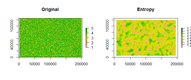
Compute focal means of the indicators of each vegetation type. At each cell, these give the proportions of the types. Multiply each by its negative logarithm and sum: that's the diversity index.

You will find that even for large numbers of categories (even into the hundreds), this is fantastically faster than the brute-force method of tabulating each neighborhood in turn, even with tiny neighborhoods. That is because it is carried out by means of convolutions, achieving O(m*n*log(m*n)) scaling for m rows and n columns, regardless of the neighborhood size. The brute-force tabulation method simply will not complete executing in any reasonable time on any rasters of meaningful size or using large neighborhoods.

The code at the end illustrates the procedure. It uses a 41 by 41 circular neighborhood on a 500 by 800 raster involving five categories; the timing is under 10 seconds. That's poor, actually: it can be improved by several of orders of magnitude on other platforms. However, it might be good enough for production work when rasters are not too large.

This code gives results that differ from vegan and from another answer in this thread. The reason is subtle: focal first multiplies all elements in the neighborhood by the focal weights and then passes all values to its function. For non-rectangular neighborhoods that introduces some zeros. Those zeros are not included in the neighborhood and therefore should not be tabulated. However, the approach using table actually does tabulate the frequencies of those zeros. The effect is to add a constant value (equal to -r *log(r) where r is the proportion of zeros in a neighborhood) except around the edges (where the neighborhood shape, and therefore r, can change).

library(raster)
m <- 500            # Rows
n <- 800            # Columns
cellsize <- 250     # Meters
p <- (1:5)^2        # Relative probabilities of vegetation; first is NoData
radius <- 5000      # Meters
#
# Create sample data.
#
set.seed(17)
x <- matrix(sample.int(length(p), m*n, replace=TRUE, prob=p), nrow=m)
#
# Convert to raster.
#
x.r <- raster(x, xmn=0, ymn=0, xmx=n*cellsize, ymx=m*cellsize)
#
# Diversity index.
#
diversity <- function(x.r, radius, type="circle", verbose=TRUE) {
  # 
  # Create focal weights matrix.
  #
  nbrhd <- focalWeight(x.r, radius, type=type)
  #
  # Compute focal means of indicators.
  #
  entropy.r <- calc(x.r, function(x) 0)
  x.log <- function(x) ifelse(x==0, 0, x*log(x))
  for (i in 1:length(p)) {
    if (verbose) cat("Computing indicator for category", i, "... ")
    z <- system.time({
      entropy.r <- entropy.r - calc(focal(x.r == i, nbrhd), x.log)
    })
    if (verbose) cat(z[3], "seconds.\n")
  }
  return (entropy.r)
}
#
# Plot the original and its entropy.
#
entropy.r <- diversity(x.r, radius)
par(mfrow=c(1,2))
plot(x.r, main="Original")
plot(entropy.r, main="Entropy")

Answer 2

Here's a simple implementation for you. Edit: fixed focal weights matrix to exclude 0s as per whuber's comments in his answer.

library(raster)

# Example Data
set.seed(1)
r <- raster(matrix(sample(1:10, 100, replace=T), 10, 10))

# Calculate a weights matrix, and reset elements to 0s and 1s 
# rather than true weights
fw <- focalWeight(r, 0.2, 'circle')
fw <- ifelse(fw == 0, NA, 1)

# Neighbourhood richness
richness <- function(x, ...) {
    length(unique(na.omit(x)))
}
richOut <- focal(r, fw, fun=richness, pad=T)

# Neighbourhood Shannon Diversity Index
shannon <- function(x, ...) {
    cnts <- table(x)
    cnts <- cnts / sum(cnts)
    -sum(cnts * log(cnts))
}
shanOut <- focal(r, fw, fun=shannon, pad=T)

The vegan package also has a diversity function that can calculate Shannon, Simpson, and Fisher diversity indices for you. The results are the same.

library(vegan)
shannonVegan <- function(x, ...) {
    diversity(table(x), index="shannon")
}
shanVegOut <- focal(r, fw, fun=shannon, pad=T)  

It occurs to me that there may be some edge effects due to the focal circle going off the edge of the grid. You could change pad=T to pad=F to get NAs for any cells where this would be an issue, or just be aware of it.