How to redistribute values of a raster according to a gaussian distribution

Question

I have a matrix of dimension 10 x 10, with each cell value equal to 100.

100 100 100 100 100 100 100 100 100 100
100 100 100 100 100 100 100 100 100 100
100 100 100 100 100 100 100 100 100 100
100 100 100 100 100 100 100 100 100 100
100 100 100 100 100 100 100 100 100 100
100 100 100 100 100 100 100 100 100 100
100 100 100 100 100 100 100 100 100 100
100 100 100 100 100 100 100 100 100 100
100 100 100 100 100 100 100 100 100 100
100 100 100 100 100 100 100 100 100 100

And I would like to create a new matrix in which these values are distributed according to a gaussian distribution with values higher than 100 in the middle of the matrix and values lower than 100 going towards the borders of the matrix.

However, I want the total sum of values to be the same in the two matrices (therefore 10.000).

Do you have any suggestion on how I could do it in R?

Answer 1

You should be clear on exactly what you are after here. It is easy to generate a random raster or matrix, following a Gaussian distribution. However, it is quite different to create a 2D Gaussian distribution following z[x,y].

Here is a general methodology to approximate what you are after. You can fool around with scaling the resulting matrix however you want.

Create 10x10 matrix of uniform values

( m <- matrix(100,nrow=10,ncol=10) )

Create Gaussian distributed matrix with a sd = 1.5

library(spatialEco)
( gm <- spatialEco::gaussian.kernel(sigma=1.5, n=10) )

Multiply matrices, this step is somewhat meaningless but, demonstrates weighting an existing matrix with a Gaussian distribution.

( wm <- m * gm )

plot results

persp(x=1:nrow(wm),y=1:ncol(wm),z=wm, col="blue")

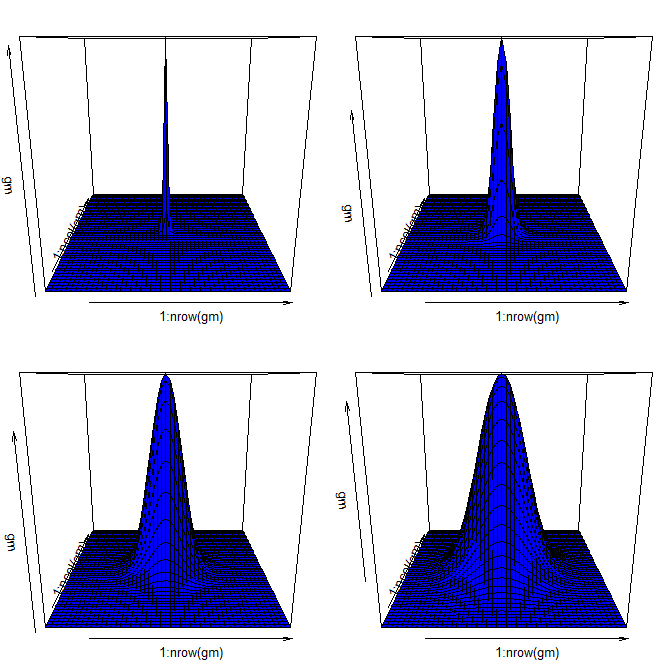
Here we can look at some different sigmas whose effect are a function of the size of the data.

par(mfrow=c(2,2), mar=c(1,0.5,0.5,0.5))     
  for(s in c(0.5, 2, 4, 6)){ 
    gm <- spatialEco::gaussian.kernel(sigma=s, n=50)        
    persp(x=1:nrow(gm),y=1:ncol(gm),z=gm, col="blue")   
  } 

In a simulation framework, you can start digging a bit deeper and simulating multivariate normal kernels. Bit off topic but, still interesting in the realm of 2D kernel estimates. We often neglect multivariate normal in thinking Gaussian normal.

Define some simulated pairwise data

nx <- 20
x <- seq(0,2,length=nx)
X <- expand.grid(x, x)

Create squared exponential kernel

D <- plgp::distance(X)
Sigma <- exp(-D/1)^2 + diag(sqrt(.Machine$double.eps), nrow(X))

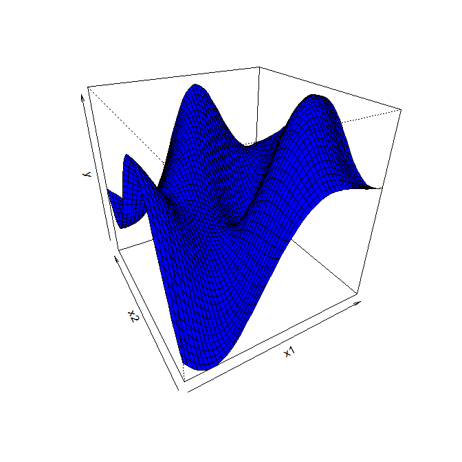
Sample from multivariate normal distribution with mean zero and specified sigma and plot the results

Y <- MASS::mvrnorm(1,rep(0,dim(Sigma)[1]), Sigma)
  persp(x=x,y=x, z=matrix(Y, ncol=nx,nrow=nx), 
        theta=-30, phi=30, xlab="x1", ylab="x2",  
        zlab="y", col="blue")