15

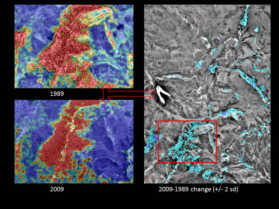
I am looking for a different, more elegant solution to a spatial statistics problem. Raw data consists of an x-y coordinate for each individual tree (i.e. converted to a point .shp file). Although not used in this example, every tree also has a corresponding polygon (i.e. as a .shp) which represents the crown diameter. The two images on the left show landscape-scale kernel density estimates (KDEs) derived from a point .shp file of individual tree locations--one from 1989 and the other from 2009. The graphic on the right shows the difference between the two KDEs where only values +/- 2 standard deviations of the mean are displayed. Arc's raster calculator was used to perform the simple calculation (2009 KDE - 1989 KDE) necessary to produce the raster overlay on the right hand image.

Is there a more appropriate method for analyzing tree density or canopy area change over time either statistically or graphically? Given these data, how would you assess the change between the 1989 and 2009 tree data in a geospatial environment? Solutions in ArcGIS, Python, R, Erdas and ENVI are encouraged.

enter image description here

5
  • 3
    Do you have the original tree location data from 1989? If not, do the KDEs at least use the same kernels (and same bandwidths)? Are the tree data a complete census of the area or are they some kind of sample (and if so, how were the members of that sample selected)? What constitutes a "change" in your study and how would you like to measure it (e.g., as an absolute change in tree density or a relative change)?
    – whuber
    Commented Jun 23, 2012 at 15:49
  • 1
    @whuber: The original tree locations can be considered census data as every tree within the DOQQ was inventoried. The KDE was based on points derived from the census data. I am primarily interested in detecting new trees and change in canopy cover.
    – Aaron
    Commented Jun 23, 2012 at 16:46
  • 1
    KDEs might be inappropriate here since change in tree location and numbers will change the bandwidth and therefore the results. Have you considered creating a zonal raster of arbitrary size (say 100m x 100m) and getting trees / cell and tree area / cell for each time and then calculating a difference between times? Commented Jun 28, 2012 at 21:35
  • @blindJesse: You have a good point. As an alternative, I've been toying around with the idea of converting the canopy diameter polygons from 2009 and 1989 to rasters, then reclassifying the rasters to binary data. From there, I can run a moving window focal statistics script on the difference between the two.
    – Aaron
    Commented Jun 28, 2012 at 23:27
  • 1
    I'm still unsure of the form of the raw data, Aaron. When you write "every tree ... was inventoried," does that mean each individual tree was identified and assigned coordinates? Or perhaps does it mean someone drew a polygon and said "I found 39 red maples and 13 white oaks inside here?" Understanding the strengths and limitations of the original data is crucial to obtaining the canonical answer you seek.
    – whuber
    Commented Jun 29, 2012 at 20:02

3 Answers 3

8
+150

First problem:

You're looking at a mixture of minima. One gigantic tree with an acre-sized crown looks quite a lot, interpreted on a point / kernel density basis, like a field with no trees at all. You will end up with high values only where there are small, rapidly growing trees, at edges and in gaps in the forest. The tricky bit is, these dense smaller trees are much more likely to be obscured by shadow or occlusion or be un-resolvable at a 1-meter resolution, or be aglomerated together because they're a clump of the same species.

Jen's answer is correct on this first part: Throwing away the polygon information is a waste. There is a complication here, though. Open-grown trees have a much less vertical, more spreading crown, all other things being equal, than an even-aged stand or a tree in a mature forest. For more see #3.

Second problem:

You should ideally be working with an apples to apples comparison. Relying on NDVI for one and B&W for the other introduces an un-knowable bias into your results. If you can't get suitable data for 1989, you might instead use degraded B&W data for 2009, or even try to measure the bias in the 2009 data relative to the B&W and extrapolate the NDVI results for 1989.

It may or may not be plausible to address this point labor-wise, but there's a decent chance it would be brought up in a peer review.

Third problem:

What precisely are you trying to measure? Kernel density isn't a value-less metric, it gives you a way to find areas of new-growth, young trees which are rapidly killing each other off (subject to the shading/occlusion limitations above); Only the ones with the best access to water/sunshine, if any, will survive in a few years. Canopy coverage would be an improvement on kernel density for most tasks, but that has problems as well: it treats a big even-aged stand of 20-year-old trees that have just barely closed the canopy as much the same as an established 100-year-old forest. Forests are hard to quantify in a way that will preserve information; A canopy height model is ideal for a lot of tasks, but impossible to get historically. The metric you use is best chosen based on an elaboration of your goals. What are they?

Edit:

The goal is sensing scrubland expansion into native grassland. Statistical methods are still perfectly valid here, they just require some elaboration and subjective choices to apply.

  • Calculate a basic measure of canopy coverage. This may involve a gridded approach directly on the crown polygons, or turning the crown polygons to a raster + blurring them if you need a more continuous version.
  • Try separating out classes of landscape in which to do your analysis, based on percent canopy coverage. The statistical techniques you work with in closed canopy forest may be different than those you use on an almost-bare grassland, or may even be defensibly excluded from the analysis. Some small area of your landscapes will include "scrubland expansion", and choosing how to subset out that effect & ignore data that isn't relevant is up to you as a statistician.
  • I don't know if this will work over a 20-year timespan (and it will work better with additional intermediate epochs), but try paying attention to crown diameter as a proxy for tree age. There's a definitional question you have to ask, whether the doubling in size of an existing crown represents "expansion", or whether it requires new trees. If it's the latter, you do have some idea whether they are new (at least, for some classes of landscape you selected out above, where you can verify a certain degree of sunlight access).
  • Depending on your ecological aims, it may be worthwhile not only to explore tree density directly, but to explore landscape fragmentation using packages like Fragstats.
  • Long shot: Make sure there's no county LIDAR dataset lying around waiting to be used as validation and accuracy assessment for your ability to distinguish crowns in the 2009 dataset.
2
  • Thanks Chris, You bring up many legitimate holes in the KDE approach to change detection. I have been struggling with how best to deal with the difference in image quality between 2009 and 1989. I agree that a training dataset is warranted to compare the imagery output. The purpose of these data is to assess shrubland expansion into native grasslands. I gather the best approach is to utilize the power of these census data and, in fact, not use a statistical approach--but rather, a descriptive one.
    – Aaron
    Commented Jul 2, 2012 at 12:53
  • Not necessarily. Answer edited with some suggestions. Commented Jul 2, 2012 at 21:23
5

The problem with your KDE appraoch is that it smoothes the whole area and thus closes gaps you might want to find.

When I read that you used NDVI for tree crown detection, I wonder how the crown-polygons look like? are these really single polygons with tree-species ID linked to it?

If you have the luxury to have polygons for every single tree crown and you are interested where a tree crown was lost, then I think there are two possibilities; a vector and a raster solution.

vector

  1. combine all polygons from one year so that no overlapping polys remain. single polys are fine. this will lead to two shapefiles
  2. use overlay or intersect to find areas where 1989 and 2009 do not match (anymore).

raster

  1. convert all polygons from each year into a binary raster with 0 = notree and 1=tree. use a high resolution, e.g. 0.5m and bilinear interpol? this will make sure that edges are smooth
  2. subtract the binary images (2009-1989) and you should get something similar to your first result but free from the smoothed KDEs

I hope that works out :) I did not try these ideas out but simply wrote down what came to my mind. good luck!

oh...maybe, you could also simply make a quadrat count approach. for each year, slice up your area using a vector grid of 100x100m, count points in polygons and compare the two different pattern. just another idea...

1
  • Jens, excellent analysis of the ecological problem. Your succinct answer both identifies a serious problem with the KDE approach and has really helped with an overall way forward.
    – Aaron
    Commented Jul 2, 2012 at 21:52
2

A general change in vegetation may be calculated using a Digital Change Analysis. To run this analysis you will first need a 4-band (R,G,B, and NIR) image for both 1989 and 2009. Next, using a remote sensing software (such as ENVI or Erdas) run a NDVI analysis on each image. NDVI analysis compares the ratio of NIR band – red band/ NIR band + red band pixels. The result of this equation gives pixel values that range from -1 to 1. Pixels that have a value of less than zero show no reflectance in the NIR band. Likewise, pixels that have a value greater than zero reflect NIR light and thus are considered vegetation. The process of performing a digital change analysis is simply subtracting one NDVI image from the other (subtract 1989 from 2009). Please see link below for a more in-depth discussion.

http://www.bioline.org.br/pdf?er07006

1
  • Thank you for a thought provoking reply and reference. NDVIs were created from 2009 1m 4-band NAIP DOQQs to derive tree locations. However, 1989 1m NAIP imagery is only available in greyscale--so these images had to be manipulated differently in order to derive tree locations. There may be too much "background noise" for this study using NDVIs generated from TM, or other low res imagery for digital change analysis. Thanks again!
    – Aaron
    Commented Jun 26, 2012 at 3:26

Your Answer

By clicking “Post Your Answer”, you agree to our terms of service and acknowledge you have read our privacy policy.

Not the answer you're looking for? Browse other questions tagged or ask your own question.