Selecting certain road length around points in QGIS

Question

I have a dataset with road segments across a country, and their length in km. I also have the boundaries of each province within the country. I have calculated the center point of each province.

What I would like to do now in QGIS is to select a contiguous % of road lengths per province, and have the selection radiate out from the center point of each province.

Here's a screenshot of what I'd like to achieve: rather than randomly selecting 10% of the roads (shown in green and orange) I have the red dot, and want to just highlight 10% of roads (by length) around the dot (as shown in blue).

Answer 1

This solution relies on two relatively new functions of QGIS expressions: array_sum(), avalilable since QGIS 3.18 and overlay_nearest(), available since QGIS 3.16.

1. Calculate the total length of the roads per province.

2. Calculate the length of the percentage you want to get. In my example, the total length is 1090566 m, 10% thus is 109056.6 m

3. Remark: see below for a more systematic calculation of what is done here with trial and error: On the point layer, now use field calculator with the following expression. It calculates the accumulated length of the x nearest road segments. In my case, x is 100 (the limit:=100 part). Change the value manually to get as close as possible to the value you need (109056.6 m in my case):

   array_sum(overlay_nearest('road', length ($geometry), limit:=100))

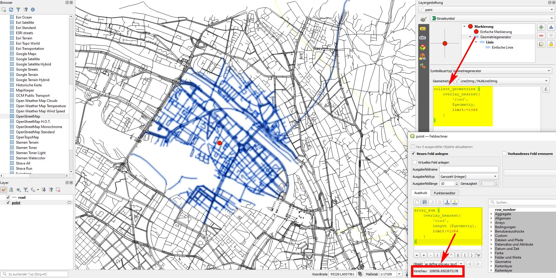
   Playing around, in my case I reach a value of accumulated road-length of 109056.85 m with a value of limit:=1064. That means: I must add the length of the 1064 road segments nearest to the point to reach the total amount I want to have.

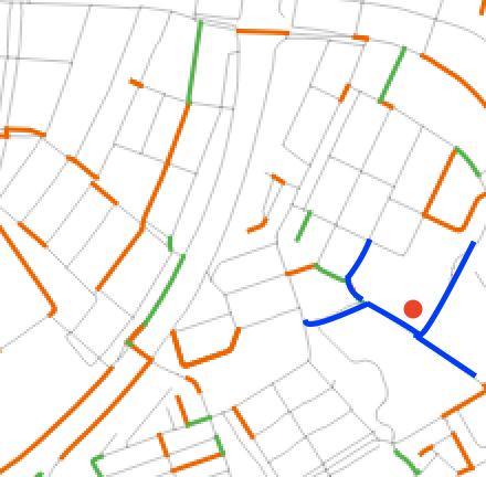
4. Now, changing the expression a little bit, I am able to display these road segments. The expression to do that: collect_geometries(overlay_nearest('road', $geometry, limit:=1064)). This can be done either with the "Geometry Generator" or the "Geometry by Expression": see here for how to do that.

Screenshot: on the lower right, see the expression that returns the value I look for in the preview. Above, see the expression used with geomtry generator (the blue lines):

Edit:

In the first version, in step 3 above you had to manually set the value to get as close as possible to the percentage value calculated in step 2. However, there is an automatic was to do so. The steps 5 to 8 that follow here replace step 3 above. Step 3 is a fast way to find the value needed in step 4. The steps that follow here are a systematic way to calculate this value. I continue the numbering of the steps starting with 5 to avoid confusion with the steps above.

5. On the point layer, create a new string attribute field called order, consisting of an array of id values: each road segment in the order of their distance to the center point: id of closest, id of second closest, id of third closest etc. Use this expression: array_to_string (overlay_nearest( 'road', $id, limit:=-1))

6. On the road layer, now assign to each road segment a new attribute with the place it appears in the order of closeness to the center point: 1 for the closest, 2 for the second closest etc. For this, access the array calculated above with attribute() and convert it's string format back to an array with string_to_array(). Than, return the index (position) each road-id has in the array with array_find(). The whole expression looks like this - use it to create a new attribute field called closeness with field calculater:

   array_find( 
       string_to_array (
           attribute (
               get_feature_by_id ('point',1), 
               `order`
           )
       )
       , $id
   )
   

7. Now calculate a new field called length_accumulated, based on the aggregated sum of the length, starting with one segment (the closest to the point), two segments (the two closest), three segments (the three closest) etc., based on the length of each segment and the order of closeness calculated before. This can be done with the following expression. With array_agg(), you aggregate the length of the segments, ordered by the closeness attribute, resulting in an array of length-values. With array_slice(), you select a subset of this array, starting with index=0 (the first element) and going up to the element with the value of the closness field. Thus for the closeness-value 10, you get a new arry with just the first eleven (0 to 10) length-values. With array_sum(), calculate the sum of the values contained in the array:

   array_sum (
       array_slice( 
           array_agg( 
               length ($geometry), 
               order_by:=closeness
           ),
           0,
           closeness
       )
   )
   

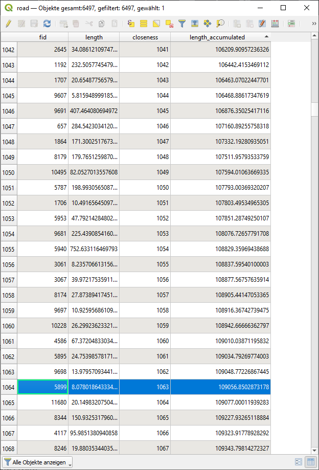
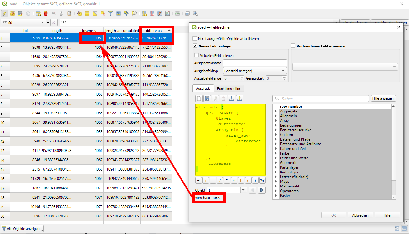
8. Now you have to find the value in the length_accumulated field that is closest to the percentage value originally calculated above in step 2. You can do it manually (screenshot 3 below) or automatize this step as well (screenshot 2). To do it, calculate a field difference that returs the absolute value of the difference of the distance you need (the one calculated in step 2) and the lenth_accumulated field: abs (109056.6- length_accumulated). If you now sort this field, the smallest one gets on top and you can read the closeness-value of 1063 (same as above). You could again use an expression that returns this value. Create an array of all difference values with array_agg(), get the smallest value with array_min(), find the feature where the difference-field has this minimum value with get_feature() and than from this feature return the value of the closeness-field with attribute(). As you can see on the right side of screenshot 3, in the preview, you get the value of 1063 that we need:

   attribute (
       get_feature (
           @layer, 
           'difference', 
           array_min (
               array_agg( 
                   difference
               )
           )
       ), 
       'closeness'
   )
   
   
   

Screenshot 2: you can sort the calculated difference-field (semi-manual solution) or again use an expression to return the value of the closeness-field that gives you the number of x closest road-segments that together have a length closest to the value you need (y% of total, as calculated in step 2):

Screenshot 3: to look up the value manually - the field length_accumulated reaches a value close to the one we need for the closeness value of 1063. As counting (based on arrays) starts from 0, we effectively have the same number of the 1064 closest road segments as above. Thus you can take this value and insert it above in step 4.