Using weight component in Moran I calculation

Question

I'm trying to understand the Moran I calculation, and there is something I don't understand. In this tutorial, Moran I described as the slope value of the correlation between one polygon to the neighbors mean value :

However, in other sources (including wikipedia), there is specific formula :

Based on this, it seems like the calculation is more complex, and also, there is spatial weight. I know about the weights that it can be for example rook or queen, and also neighbor degree, but I don't understand how that being expressed in this formula.

What is the weight component and how is it being expressed in the formula as number?

Answer 1

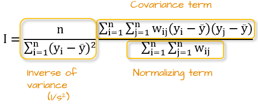
The source of confusion may be in the two W terms in your equation--this may suggest different types of weights in the formula. It will therefore be helpful to re-express the Moran’s I equation in a different form as follows:

Using the dataset you reference in your post as an example, y_i is the income for a polygon of interest, i, and y_j is the income for all other polygons, j, in the dataset. y^bar is the mean income values for all polygons in the dataset. The weight w_ij is 0 if polygon j is not a neighbor of polygon i. If polygon j is a neighbor of polygon i, then the weight w_ij takes on a non-zero value. This non-zero value can vary depending on how a neighbor’s weight is defined. n is the total number of polygons.

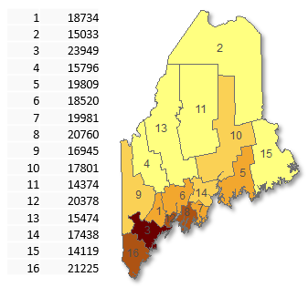
To understand how the weights are used in the formula, we’ll work with the example you share. The map of the 16 polygons along with the income values are shown in the following figure.

The first step in the workflow is to conceptualize the idea of a neighbor. This can be contiguous polygons, distance between centroids, kth neighbors, etc…

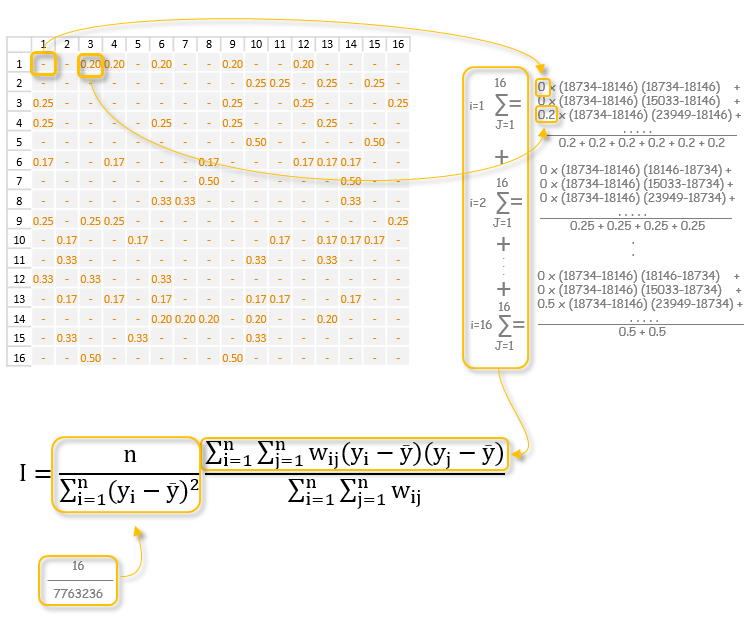
The next step is to compute the neighborhood matrix. Here, all polygons are represented in both the rows and columns. The i^th polygons are listed along the rows, the j^th polygons along the columns. The intersection of the two is the weight the polygon in the j^th column contributes to the neighboring polygons of the i^th row. The weight values can be computed in many different ways. For example, the values can be binary (1 for neighboring polygons and 0 otherwise), or fractions where the sum of each neighboring polygon fraction sums to one—-this gives us the mean value of the neighboring polygons, for example. The figure below adopts the latter matrix computation.

Once the weight matrix is computed, its weight values are used to compute the Moran’s I value. The weights are used in both the numerator and the denominator as shown in the following figure.