Create polygon grid based on spatial points (WGS84) with R

Question

Initial problem: I am currently trying to create a spatial grid in which each cell is centered on predefined spatial points. These spatial points are projected in the WGS84 international coordinate system.

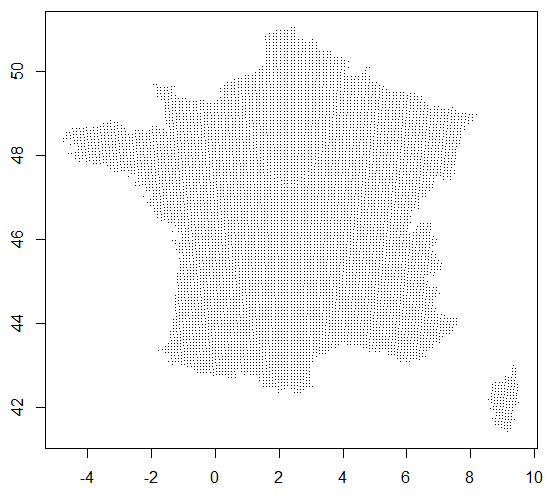
I am starting with a long/lat dataframe containing around 8000 point-location over France (data available here).

df=read.table("~/centroids.csv",sep=",",header=T)
plot(df$longitude,df$latitude,pch=".")

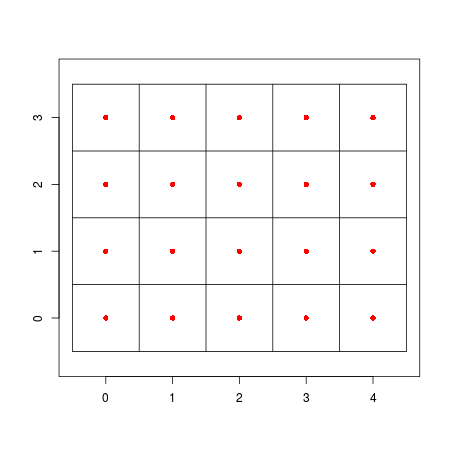
I want to compute "tile" polygons that will fill the entire space around these points. Something like in this post, with each point of df at the center of tiles, such as :

I tried several methods from the sf and raster package such as : st_make_grid(), rasterFromXYZ() combined with rasterToPolygons() that I saw in this post, or even the basic raster() using gridded() that I saw on this post. I also tried to use gBuffer() such as in this post. But without any sucess... I am always fighting against projection or non-regular/planar coordinates errors !

Once I will be able compute those tiles (or polygons), I want to store them in a simple feature object (from the sf package). Within this sf object: each polygon will correspond to a cell of the final spatial grid; each polygon will be centered on a spatial point from df; and each polygon will inherit the ID of the point (from df) on which it is centered.

Is that possible ???

Answer 1

Final solution:

library("sp")
library("sf")
library("raster")
library("parallel")
library("ggplot2")

df=read.table("~/centroids.csv",sep=",",header=TRUE)

df2=df
coordinates(df2)=~longitude+latitude
proj4string(df2)=CRS("+init=epsg:4326") # points are initially projected in WGS84
df2=spTransform(df2,CRS("+init=epsg:27572")) # points are distributed on an approximatly regular grid in NTF Lambert Zone II (thank you @FSimardGIS !!!)

grid=points2grid(df2,tolerance=0.00587692) # 0.00587692 is the minimum value I found by hand, by trial and error
grid=as.data.frame(SpatialGrid(grid)) 
coordinates(grid)=~longitude+latitude

grid=rasterFromXYZ(grid)
grid=rasterToPolygons(grid)
grid=st_as_sf(grid)
st_crs(grid)=27572
grid=st_transform(grid,crs="+init=epsg:4326") # re-projection of the grid in the initial projection of df values which are in WGS84

cl=makeCluster(spec=(detectCores()-1)) # parallel computation in order to know which cells from grid actually contain points from df
clusterEvalQ(cl,library("sf"))
clusterExport(cl,c("grid","df"))
df$gridLoc=parApply(cl,df,1,function(row){
  pnt=st_sfc(st_point(c(row["longitude"],row["latitude"])),crs=4326)
  id=row["ID"]
  return(as.numeric(st_intersects(pnt,grid)))
})
stopCluster(cl)

grid=grid[df$gridLoc,] # selection of cells from grid that actually contain points from df
grid$layer=df$ID # transfert the ID of centroids to the coresponding cell of the grid

x11()
ggplot()+
  geom_sf(aes(fill=layer),col="black",data=grid)+
  geom_point(aes(x=longitude,y=latitude),pch=21,fill="white",col="black",size=.9,data=df)+
  scale_fill_gradient2(low="#47fe44",mid="#f8fe44",high="#fe4444",midpoint=5000)

Which give this nice plot (color layer corresponds to the initial ID of spatial points in df, white dots correspond to the initial centroids from df):

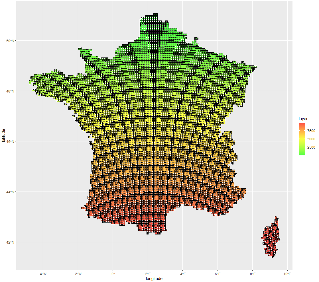
Even if some points seem to be a bit off-center from the cell, its only a plotting artifact due to the high resolution, as we can see here with increased zoom on Corsica:

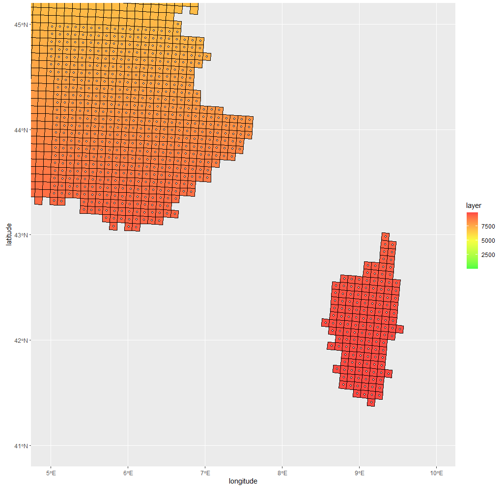
The answer to this post is therefore : (1) find the right projection in which points form a regular grid; (2) use gridded() or points2grid() to compute the regular grid; (3) transform the grid points into a raster using rasterFromXYZ(); (4) transform the raster into polygons using rasterToPolygons(); (5) re-project the polygons into the initial projection using st_transform(); (6 optional) if you do not want to keep all created cells within the grid, use st_intersects() to find which cells actually contains initial points.

Thanks a lot for your advices !

Testing the grid centroid offsets: I can compute the centroids of the grid and compare their location to the initial centroids:

estimatedCentroids=st_centroid(grid) # new centroids from grid

coordinates(df)=~longitude+latitude
proj4string(df)=CRS("+init=epsg:4326")
trueCentroids=st_centroid(st_as_sf(df)) # initial centroids from df

centroidsOffset=st_distance(estimatedCentroids,trueCentroids,by_element=TRUE) # compute distance of each pair of centroids between grid and df

hist(centroidsOffset,nclass=100)

With the final solution that I present above, I therefore make an average error of 550m (range from 170m to 900m):

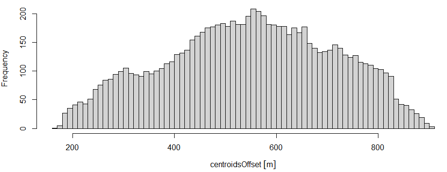
If I well understand the methodology, this is due to the use of the points2grid() function with a tolerance parameter of 0.00587692. Which means that points are not distributed on a true regular grid, even in the NTF Lambert Zone II projection (which still the better I found).