Slope calculation with datasets in different CRS

Question

I have a shapefile containing several zones. This file is in CRS EPSG:32644 (WGS 84 / UTM zone 44N).

I have a DEM file (originally in CRS EPSG:4326 - WGS 84) that I converted to EGM08. The elevation units of this converted file are in meters.

I now want to calculate the slope file for this DEM file so that I can later use the zonal statistics from my first file with the slope values.
To calculate the slope values, I tried gdaldem (https://gdal.org/programs/gdaldem.html), however this assumes that "x, y and z units are identical". This I think is not the case and since my DEM coordinates aren't close to the equator it is suggested to reproject the file.

To what projection exactly should I reproject my DEM file to obtain the least distorted values for the slope?

Answer 1

Assuming EPSG:32644 is a decent coordinate system for your DEM, then I'd use that.

Your DEM is a gridded approximation to the actual ground surface and there's probably more noise in that approximation than in the transform-and-compute-slope calculation.

If you have other projected coordinate systems that work in your study area, you could try all of them and then sample the slope calculations at a set of points for each projected DEM to see how much variability there is, and then you can decide if that is acceptable for your use case.

As an exercise I took a DEM I had which was in EPSG:3035, a standard European CRS, then warped it to lat-long (4326) then warped that to three new rasters: 27700 (standard british grid) 32630 (UTM zone for the UK) and back to 3035, to see what the round trip from 3035-LatLong-3035 would do. All conversions were done via gdalwarp on the command line with default options.

Then each raster was read (using R) and slope variable computing (using R's terra package). From the slope raster, 100 identical locations were samples scattered across the raster. The locations were specified in lat-long but converted to each slope raster coordinate system for sampling (since the grids don't align after all this warping, using 100 scattered points seems reasonable).

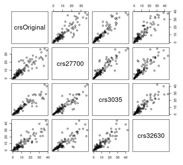
The following scatterplot matrix shows all pairs of corresponding slopes at the 100 locations.

All plots show a reasonable 1:1 trend, with only really large differences in estimated slope showing at large slope values in most cases.

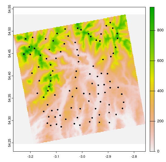
Here's the lat-long DEM and the 100 sample points for reference. The DEM is skewed because this is warped from the "original" in 3035 coordinates (and its possible I made that from a lat-long original, I just found it hanging around on my drive):

This would make a nice student project, and there's probably also a load of research into this too. This could all be done in QGIS with a lot of clicking, I did it in 10 lines of R code.

Answer 2

I would suggest transforming your vector data, and computing slope on the original lon/lat raster data

library(terra)
f <- system.file("ex/elev.tif", package="terra")
r <- rast(f)
r
#class       : SpatRaster 
#dimensions  : 90, 95, 1  (nrow, ncol, nlyr)
#resolution  : 0.008333333, 0.008333333  (x, y)
#extent      : 5.741667, 6.533333, 49.44167, 50.19167  (xmin, xmax, ymin, ymax)
#coord. ref. : lon/lat WGS 84 (EPSG:4326) 
#source      : elev.tif 
#name        : elevation 
#min value   :       141 
#max value   :       547 

x <- terrain(r, "slope")
plot(x)

And transform your polygons to the crs of the raster data to extract the zonal values.