55

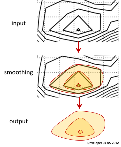
Here is a contour map for which all the polygons of levels are available.

Let ask how to smooth the polygons keeping all vertices preserved in their exact locations?

Indeed the contour is made on top of a grid data, you may suggest then to smooth the grid data and hence the resulting contour will be smoother. Note that this is not working as my desire since the smoothing function such as Gaussian filter will remove small packs of data and will change the range of the third variable e.g., the height which are not allowed in my application.

Actually I'm looking for a piece of code (preferably in Python) which can do the smoothing of 2D polygons (any type: convex, concave, self-intersecting etc) reasonably painless (forget pages of codes) and accurate.

FYI, there is a function in ArcGIS that does this perfectly, but using third party commercial applications is not my choice for this question.
enter image description here


1)

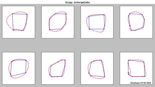
Scipy.interpolate:

enter image description here

As you see the resulting splines (red) are not satisfactory!

2)

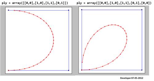
Here is the result using the code given in here. It is not working well!
enter image description here

3)

To me the best solution should be something like the following figure in which a square is being smoothed gradually by changing only one value. I hope for similar concept for smoothing any form of polygons.
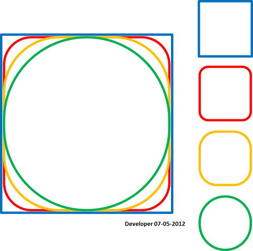
enter image description here

Satisfying the condition that spline passes the points:
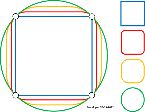
enter image description here

4)

Here is my implementation of "whuber's idea" line by line in Python on his data. There are possibly some bugs since the results are not good.
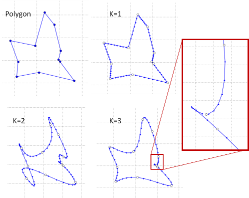
enter image description here

K=2 is a disaster and so for k>=4.

5)

I removed one point in the problematic location and the resulting spline is now identical to whuber's. But it is still a question that why the method does not work for all cases?
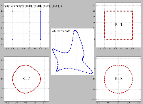
enter image description here

6)

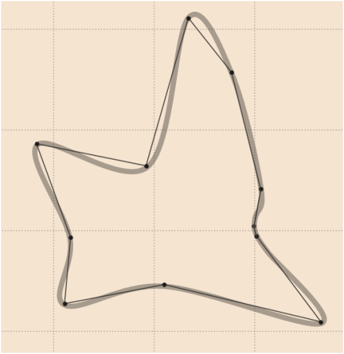
A good smoothing for whuber's data can be as follows (drawn by vector graphics software) in which an extra point has been smoothly added (compare with update

4):
enter image description here

7)

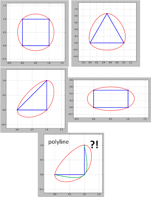
See the result from Python version of whuber's code for some iconic shapes:
enter image description here
Note that the method seems doesn't work for polylines. For the corner polyline (contour) green is what I want but got red. This needs to be addressed since contour maps are always polylines although closed polylines can be treated as polygons as in my examples. Also not that the problem emerged in update 4 has not been addressed yet.

8) [my last]

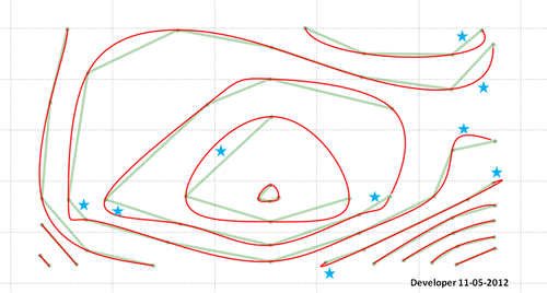
Here is the final solution (not perfect!):
enter image description here

Remember that you will have to do something about the area pointed by stars. There is perhaps a bug in my code or the proposed method needs further development to consider all situations and to provide desired outputs.

22
  • how are you generating 'polygon' contours? wouldn't they always be lines, since a contour intersecting the edge of a DEM would never close upon itself? Commented May 5, 2012 at 5:14
  • i've used the v.generalize function in GRASS to do smoothing of contour lines with decent results, although it can take awhile for maps with very dense contours. Commented May 5, 2012 at 5:24
  • @pistachionut You may consider the contour levels are poly-lines. I'm looking for pure code at the first stage. If not available then light package for Python.
    – Developer
    Commented May 5, 2012 at 5:36
  • Perhaps look at scipy.org/Cookbook/Interpolation because it sounds like you want to spline
    – PolyGeo
    Commented May 6, 2012 at 7:13
  • 1
    @Pablo Bezier curve in your link works well for polylines. whuber's works almost well for polygons. So they together could address the question. Thanks a lot for sharing your knowledge for free.
    – Developer
    Commented May 10, 2012 at 11:25

3 Answers 3

38

Most methods to spline sequences of numbers will spline polygons. The trick is to make the splines "close up" smoothly at the endpoints. To do this, "wrap" the vertices around the ends. Then spline the x- and y-coordinates separately.

Here is a working example in R. It uses the default cubic spline procedure available in the basic statistics package. For more control, substitute almost any procedure you prefer: just make sure it splines through the numbers (that is, interpolates them) rather than merely using them as "control points."

#
# Splining a polygon.
#
#   The rows of 'xy' give coordinates of the boundary vertices, in order.
#   'vertices' is the number of spline vertices to create.
#              (Not all are used: some are clipped from the ends.)
#   'k' is the number of points to wrap around the ends to obtain
#       a smooth periodic spline.
#
#   Returns an array of points. 
# 
spline.poly <- function(xy, vertices, k=3, ...) {
    # Assert: xy is an n by 2 matrix with n >= k.

    # Wrap k vertices around each end.
    n <- dim(xy)[1]
    if (k >= 1) {
        data <- rbind(xy[(n-k+1):n,], xy, xy[1:k, ])
    } else {
        data <- xy
    }

    # Spline the x and y coordinates.
    data.spline <- spline(1:(n+2*k), data[,1], n=vertices, ...)
    x <- data.spline$x
    x1 <- data.spline$y
    x2 <- spline(1:(n+2*k), data[,2], n=vertices, ...)$y

    # Retain only the middle part.
    cbind(x1, x2)[k < x & x <= n+k, ]
}

To illustrate its use, let's create a small (but complicated) polygon.

#
# Example polygon, randomly generated.
#
set.seed(17)
n.vertices <- 10
theta <- (runif(n.vertices) + 1:n.vertices - 1) * 2 * pi / n.vertices
r <- rgamma(n.vertices, shape=3)
xy <- cbind(cos(theta) * r, sin(theta) * r)

Spline it using the preceding code. To make the spline smoother, increase the number of vertices from 100; to make it less smooth, decrease the number of vertices.

s <- spline.poly(xy, 100, k=3)

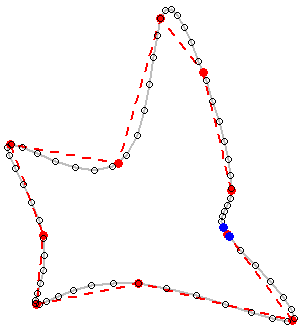
To see the results, we plot (a) the original polygon in dashed red, showing the gap between the first and last vertices (i.e., not closing its boundary polyline); and (b) the spline in gray, once more showing its gap. (Because the gap is so small, its endpoints are highlighted with blue dots.)

plot(s, type="l", lwd=2, col="Gray")
lines(xy, col="Red", lty=2, lwd=2)
points(xy, col="Red", pch=19)
points(s, cex=0.8)
points(s[c(1,dim(s)[1]),], col="Blue", pch=19)

Splined polygon

10
  • 6
    Nice answer. Is there any way to guarantee contours don't end up crossing as a result of smoothing? Commented May 7, 2012 at 20:50
  • 1
    That's a good question, @Kirk. I am not aware of any method to guarantee non-crossing from this form of smoothing. (In fact, I don't even see how to guarantee that the smoothed polyline is non-self-intersecting. This is not a big issue for most contours though.) In order to do that, you would need to return to the original DEM and instead use a better method to compute the contours in the first place. (There are better methods--they have been known for a long time--but AFAIK some of the most popular GISes do not use them.)
    – whuber
    Commented May 7, 2012 at 21:01
  • First, I am still working to implement your answer in Python, yet not successful. Second, what will be the resulting if you apply your method on a square? You may refer to those I've drawn in the question.
    – Developer
    Commented May 8, 2012 at 2:05
  • 1
    I accepted this as answer since it gives a good solution. Even though it is not a perfect one but it gave me some ideas working around, hope I'll find a solution that satisfies the points I mentioned above in my question and comments. You also may consider whuber's comments for the question [QC], there are good tricks there. Lastly I should say the translation to python is almost straightforward having lovely Scipy package installed. Also consider Pablo's comment in QC as possible solution for polylines, i.e., Bezier curves. Good luck everyone.
    – Developer
    Commented May 10, 2012 at 11:22
  • 1
    seeing your answers, I regret not taking care of my maths well!!!
    – vinayan
    Commented May 11, 2012 at 11:51
3

I know this is an old post, but it showed up on Google for something I was looking for, so I thought I'd post my solution.

I don't see this as a 2D curve fitting exercise, but rather a 3D one. By considering the data as 3D we can ensure that the curves never cross one another, and can use information from other contours to improve our estimate for the current one.

The following iPython extract uses cubic interpolation provided by SciPy. Note that the z values I've plotted aren't important, as long as all the contours are equidistant in height.

In [1]: %pylab inline
        pylab.rcParams['figure.figsize'] = (10, 10)
        Populating the interactive namespace from numpy and matplotlib

In [2]: import scipy.interpolate as si

        xs = np.array([0.0, 0.0, 4.5, 4.5,
                       0.3, 1.5, 2.3, 3.8, 3.7, 2.3,
                       1.5, 2.2, 2.8, 2.2,
                       2.1, 2.2, 2.3])
        ys = np.array([0.0, 3.0, 3.0, 0.0,
                       1.1, 2.3, 2.5, 2.3, 1.1, 0.5,
                       1.1, 2.1, 1.1, 0.8,
                       1.1, 1.3, 1.1])
        zs = np.array([0,   0,   0,   0,
                       1,   1,   1,   1,   1,   1,
                       2,   2,   2,   2,
                       3,   3,   3])
        pts = np.array([xs, ys]).transpose()

        # set up a grid for us to resample onto
        nx, ny = (100, 100)
        xrange = np.linspace(np.min(xs[zs!=0])-0.1, np.max(xs[zs!=0])+0.1, nx)
        yrange = np.linspace(np.min(ys[zs!=0])-0.1, np.max(ys[zs!=0])+0.1, ny)
        xv, yv = np.meshgrid(xrange, yrange)
        ptv = np.array([xv, yv]).transpose()

        # interpolate over the grid
        out = si.griddata(pts, zs, ptv, method='cubic').transpose()

        def close(vals):
            return np.concatenate((vals, [vals[0]]))

        # plot the results
        levels = [1, 2, 3]
        plt.plot(close(xs[zs==1]), close(ys[zs==1]))
        plt.plot(close(xs[zs==2]), close(ys[zs==2]))
        plt.plot(close(xs[zs==3]), close(ys[zs==3]))
        plt.contour(xrange, yrange, out, levels)
        plt.show()

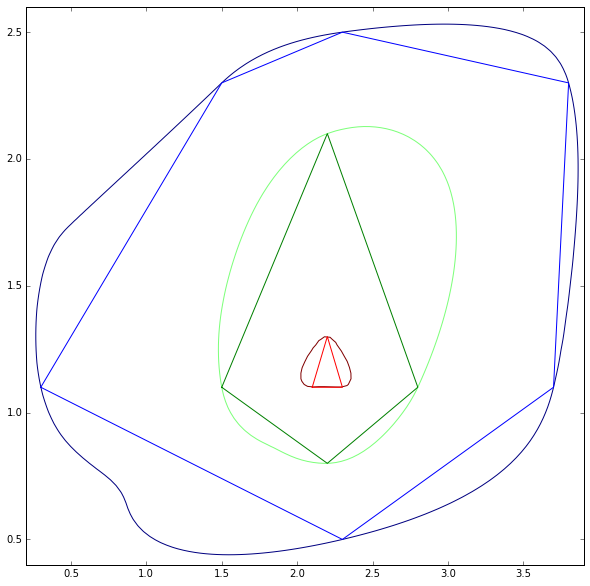
Cubic Interpolated Result

The results here don't look the best, but with so few control points they are still perfectly valid. Note how the green fitted line is pulled out to follow the wider blue contour.

1
  • 1
    The fitted smooth curves should stay close as possible to the original polygon / polyline.
    – Developer
    Commented Feb 28, 2017 at 18:23
1

I wrote almost exactly the package you are looking for... but it was in Perl, and was over a decade ago: GD::Polyline. It used 2D cubic Bezier curves, and would "smooth" an arbitrary Polygon or "Polyline" (my name then for what is now commonly called a "LineString").

The algorithm was two steps: given the points in the Polygon, add two Bezier control points between every point; then call a simple algorithm to make a piecewise approximation of the spline.

The second part is easy; the first part was a bit of art. Here was the insight: consider a "control segment" a Vertex N: vN. The control segment was three co-linear points: [cNa, vN, cNb]. The center point was the vertex. The slope of this control seg was equal to the slope from Vertex N-1 to Vertex N+1. The length of the left portion of this segment was 1/3 the length from Vertex N-1 to Vertex N, and the length of the right portion of this segment was 1/3 the length from Vertex N to Vertex N+1.

If the original curve was four vertices: [v1, v2, v3, v4] then the each vertex now get a control segment of the form: [c2a, v2, c2b]. String these together like this: [v1, c1b, c2a, v2, c2b, c3a, v3, c3b, c4a, v4] and munch them four at a time as the four Bezier points: [v1, c1b, c2a, v2], then [v2, c2b, c3a, v3], and so on. Because [c2a, v2, c2b] were co-linear, the resulting curve will be smooth at each vertex.

So this also meets your requirement to parameterize the "tightness" of the curve: use a smaller value than 1/3 for a "tighter" curve, a larger one for a "loopier" fit. In either case, the resulting curve always passes through the original given points.

This resulted in a smooth curve that "circumscribed" the original Polygon. I also had some way to "inscribe" a smooth curve... but I don't see that in the CPAN code.

Anyway, I don't at this time have a version available in Python, nor do I have any figures. BUT... if/when I do port this to Python, I'll be sure to post here.

1
  • Cannot evaluate the Perl code, add graphics to demonstrate how it was working if possible.
    – Developer
    Commented Feb 28, 2017 at 18:24

Your Answer

By clicking “Post Your Answer”, you agree to our terms of service and acknowledge you have read our privacy policy.

Not the answer you're looking for? Browse other questions tagged or ask your own question.