Statistical tests for spatial line patterns?

Question

There are plenty of tests for spatial point patterns that can be used to determine if points are distributed randomly or not, but are there any established tests for spatial line patterns? (I'm thinking straight lines, with just start and end point and no intermediate nodes.)

The data I want to analyze are OD (origin-destination) lines of human and animal movement. (Similar to the example in Clustering undirected lines.)

So far, one idea was to treat lines like 4D points and use point pattern tests but I'm uncertain if that is appropriate.

The ideal test would make it possible to determine whether there are clusters of lines or not.

Instinctively, I would say that many lines that start at the same origin but have all kinds of different destinations, should not be considered a cluster. On the other hand, many lines that run (close to) parallel for a longer time would be a cluster.

Answer 1

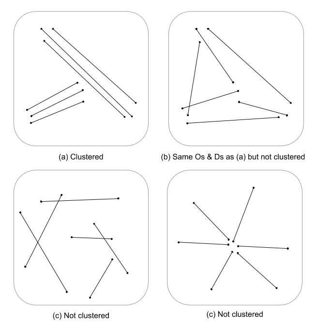
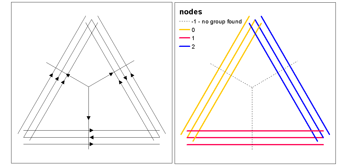
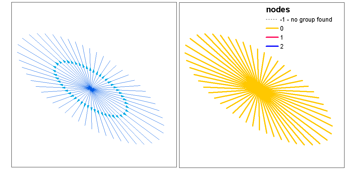
This is a difficult question as there just have not been many, if any, spatial process statistics developed for line features. Without seriously digging into equations and code, point process statistics are not readily applicable to linear features and thus, statistically invalid. This is because the null, that a given pattern is tested against, is based on point events given a random field and not linear dependencies. I have to say that I do not even know what the null would be as far as intensity and arrangement/orientation would be even more difficult.

I am just spit-balling here but, I am wondering if a multi-scale evaluation of line density coupled with Euclidean distance (or Hausdorff distance if lines are complex) would not indicate a continuous measure of clustering. This data could then be summarized to the line vectors, using variance to account for disparity in lengths (Thomas 2011), and assigned a cluster value using a statistic such as K-means. I know that you are not after assigned clusters but the cluster value could partition degrees of clustering. This would, obviously, require an optimal fit of k so, arbitrary clusters are not assigned. I am thinking that this would be an interesting approach in evaluating edge structure in graph theoretical models.

Here is a worked example in R, sorry, but it is faster and more reproducible than providing a QGIS example, and is more in my comfort zone:)

Add libraries and use copper psp object from spatstat as line example

library(spatstat)
library(spatstat.core)
library(raster)
library(spatialEco)

data(copper)
l <- copper$Lines
l <- rotate.psp(l, pi/2)

Calculate standardized 1st and 2nd order line density and then coerce to raster class objects

d1st <- density(l)
  d1st <- d1st / max(d1st)
  d1st <- raster(d1st)  
d2nd <- density(l, sigma = 2)
  d2nd <- d2nd / max(d2nd)
  d2nd <- raster(d2nd)  

Standardize 1st and 2nd order density in to a scale-integrated density

d <- d1st + d2nd
d <- d / cellStats(d, stat='max')  

Calculate standardized inverted euclidean distance and coerce to raster class

euclidean <- distmap(l)
euclidean <- euclidean / max(euclidean)
euclidean <- raster.invert(raster(euclidean))

Coerce spatstat psp to a sp SpatialLinesDataFrame object to use in raster::extract

as.SpatialLines.psp <- local({
     ends2line <- function(x) Line(matrix(x, ncol=2, byrow=TRUE))
     munch <- function(z) { Lines(ends2line(as.numeric(z[1:4])), ID=z[5]) }
     convert <- function(x) {
        ends <- as.data.frame(x)[,1:4]
        ends[,5] <- row.names(ends)
        y <- apply(ends, 1, munch)
        SpatialLines(y)
     }
     convert
})
l <- as.SpatialLines.psp(l)
l <- SpatialLinesDataFrame(l, data.frame(ID=1:length(l)) )

Plot results

par(mfrow=c(2,2))
  plot(d1st, main="1st order line density")
    plot(l, add=TRUE)
  plot(d2nd, main="2nd order line density")
    plot(l, add=TRUE) 
  plot(d, main="integrated line density")
    plot(l, add=TRUE)   
  plot(euclidean, main="euclidean distance")
    plot(l, add=TRUE) 

Extract raster values and calculate summary statistics associated with each line

l.dist <- extract(euclidean, l)
l.den <- extract(d, l)
l.stats <- data.frame(min.dist = unlist(lapply(l.dist, min)),
                      med.dist = unlist(lapply(l.dist, median)),
                      max.dist = unlist(lapply(l.dist, max)),
                      var.dist = unlist(lapply(l.dist, var)),
                      min.den = unlist(lapply(l.den, min)),
                      med.den = unlist(lapply(l.den, median)),
                      max.den = unlist(lapply(l.den, max)),
                      var.den = unlist(lapply(l.den, var)))

Use cluster silhouette values to evaluate optimal k (number of clusters), with the optimal.k function, then assign cluster values to lines. We can then assign colors to each cluster and plot on top of the density raster.

clust <- optimal.k(scale(l.stats), nk = 10, plot = TRUE)                      
  l@data <- data.frame(l@data, cluster = clust$clustering) 
 
kcol <- ifelse(clust$clustering == 1, "red", "blue")
plot(d)
  plot(l, col=kcol, add=TRUE)

At this point one could perform a randomization of the lines to test if the resulting intensity and distance are significant from random. You could use the "rshift.psp" function to randomly reorient your lines. You could also just randomize the start and stop points and recreate each line.

One also wonders "what if" you just performed a point pattern analysis using a univariate or cross analysis statistic on the start and stop points, invariant of the lines. In a univariate analysis you would compare the results of the start and stop points to see if there consistency in clustering between the two point patterns. This could be done via a f-hat, G-hat or Ripley's-K-hat (for unmarked point processes). Another approach would be a Cross analysis (eg., cross-K) where the two point processes are tested simultaneously by marking them as [start,stop]. This would indicate the distance relationships in the clustering process between the start and stop points. However, spatial dependency (nonstaionarity) on an underlying intensity process can be an issue in these types of models making them inhomogeneous and requiring a different model. Ironically, inhomogeneous process is modeled using an intensity function which, brings us full circle back to density thus, supporting the idea of using a scale-integrated density as a measure of clustering.

Here is a quick worked example of if the Ripleys K (Besags L) statistic for autocorrelation of an unmarked point process using the start, stop locations of a line feature class. The last model is a cross-k using both start and stop locations as a nominal marked process.

library(spatstat)
library(spatstat.core)
library(spatstat.geom)
  data(copper)
  l <- copper$Lines
  l <- rotate.psp(l, pi/2)

Lr <- function (...) {
 K <- Kest(...)
  nama <- colnames(K)
   K <- K[, !(nama %in% c("rip", "ls"))]
   L <- eval.fv(sqrt(K/pi)-bw)
  L <- rebadge.fv(L, substitute(L(r), NULL), "L")
 return(L)
}

### Ripley's K ( Besag L(r) ) for start locations
start <- endpoints.psp(l, which="first")
marks(start) <- factor("start")
W <- start$window
area <- area.owin(W)
lambda <- start$n / area
 ripley <- min(diff(W$xrange), diff(W$yrange))/4
   rlarge <- sqrt(1000/(pi * lambda))
     rmax <- min(rlarge, ripley)
       bw=seq(0, rmax, by=1)
( Lenv <- plot( envelope(start, fun="Lr", r=seq(0, rmax, by=1), nsim=199, nrank=5) ) )

### Ripley's K ( Besag L(r) ) for end locations
stop <- endpoints.psp(l, which="second")
  marks(stop) <- factor("stop")
W <- stop$window
area <- area.owin(W)
lambda <- stop$n / area
 ripley <- min(diff(W$xrange), diff(W$yrange))/4
   rlarge <- sqrt(1000/(pi * lambda))
     rmax <- min(rlarge, ripley)
       bw=seq(0, rmax, by=1)
( Lenv <- plot( envelope(start, fun="Lr", r=seq(0, rmax, by=1), nsim=199, nrank=5) ) )

### Ripley's Cross-K ( Besag L(r) ) for start/stop
sdata.ppp <- superimpose(start, stop)
( Lenv <- plot(envelope(sdata.ppp, fun="Kcross", r=bw, i="start", j="stop", nsim=199,nrank=5, 
                 transform=expression(sqrt(./pi)-bw), global=TRUE) ) )
             

References

Thomas J.C.R. (2011) A New Clustering Algorithm Based on K-Means Using a Line Segment as Prototype. In: San Martin C., Kim SW. (eds) Progress in Pattern Recognition, Image Analysis, Computer Vision, and Applications. CIARP 2011. Lecture Notes in Computer Science, vol 7042. Springer, Berlin, Heidelberg

Answer 2

You might want to look into Fréchet distance. I only recently found out about this after a recent question looking for a python implementation.

This is a metric for finding spatial similarity of linestrings. It's a similar idea to Hausdorff distance, the equivalent for polygon similarity measures, but for linestrings with a direction.

The Fréchet distance is defined as the minimal length of a leash connecting a dog on one trajectory with its owner on a second trajectory, both never moving backwards

This metric will have a small value for two curves which are closely located, nearly parallel, aligned the same way, and with a similar length.

That doesn't answer the cluster identification part, though.

There's a comprehensive presentation here. Your situation sounds like some of the use-cases mentioned in sections 46-49

This metric has a lot of non-geospatial usages such as

• detecting common subpatterns in gene sequencing
• handwriting recognition
• detecting correlated periods in time series like stock price histories

so while a lot of papers in the bibliography cover this topic, most of them are not geospatial. Also most of these papers come under algorithmics / mathematics / computer science rather than geospatial / geosciences and are aimed accordingly.

However this paper looked promising:-

Buchin, K., Buchin, M., and Wang, Y. (2009). Exact algorithms for partial curve matching via the Fréchet distance. In Proceedings of the 20th ACM-SIAM Symposium on Discrete Algorithms, pages 645–654

Some of the other papers sound closer in intent to what you're after - cluster identification and allocation of trajectories to clusters - but they are illustrated using time series data or other non-geospatial examples. However they might point in interesting directions.

Answer 3

I am suggesting to use approach similar to one explained here.

ALGORITHM and naming:

a) Name line layer NODES. Compute bearings

b) spatially join to itself (one to many) using distance tolerance. Name layer LINKS

c) remove from LINKS joins to itself, i.e. NAME=NAME_1

d) inside LINKS find "same" direction pairs. I used:

def theSame(aList,tol):
    maxB=max(aList);minB=min(aList)
    if abs(maxB-minB)<tol:return 1
    if abs(maxB-minB-180)<tol:return 1
    return 0
#-----------
theSame( [!BEARING!, !BEARING_1!],15)

i.e. assumed lines going in opposite direction being similar in terms of direction

d) remove non similar (0) pairs from LINKS.

e) compute groups of LINKS connected through NODES and transfer group numbers to NODES table:

Unfortunately:

However simple statistics of bearings within the group, e.g. standard deviation of:

abs(tan(bearing))

shown no deviation in first case and a very big one in second. Similarly statistics of lengths could help with 'running in parallel for a long time'.

If above is of interest I can update answer with the script that computes connected groups of links. It is using arcpy and networkx module.

Don't know how to treat pair of lines going from the same point in opposite directions...

Answer 4

There is in my eyes a problem with the definition of the lines, one that will determine what approaches to use ( some of those mentioned above). If these are OD pairs, and the geometry does not play a role, I would approach this based on network clustering. You say the networks do not form a network - so be it, but it is likely that the origins and destinations fall into meaningful regions, and thus you can treat it as a network.

If the geometry has something to say ( these are , say GPS trajectories and you want to consider the geometry), than you will need to really work in a (x,y,t) space - similar geometry of the movement footprint but at different times may not be evaluated as the same - this is not specified in the question.

Some possibilities what you can look at:

1. Closest to your need is Dodge, Weibel, Forootan (2009), here http://orca.cf.ac.uk/94865/1/PhysicsMovement.pdf
2. If geometry can be simplified, maybe the parameters mentioned here may be of use: http://www.tandfonline.com/doi/full/10.1080/17445647.2017.1313788

But finally, re-reading once more your initial question, it could be simpler: can you compute pairwise (between segments) the distance between the intersection of the linear extension of the segments and their nearest points, normalise somehow ( maybe based on the length of the segment itself) and use a matrix clustering algorithm? Reasoning: segments that intersect far are more similar (parallel) than those that intersect close by. In the drawings, you do not say how to treat co-linear, or parallel segments that are in an offset (long frechet dist). I assume that this would give troubles to the solution above. (edited for clarity, by explicitly stating "linear extension" above)

Note (Jan 2018): I have recently stumbled upon this:

1. Cai, Yuhan, and Raymond Ng. "Indexing spatio-temporal trajectories with Chebyshev polynomials." Proceedings of the 2004 ACM SIGMOD international conference on Management of data. ACM, 2004.

Which relates to trajectory similarity and thus would enable similarity quantification to some extent. This is based on polynomial approximation of curves and computing a Chebyshev distance.

Answer 5

Can you give a bit more detail on the type of data you are working with? Are these just a series of disjunct lines or do they form a network? Have you used any of the ArcGIS tools for spatial pattern analysis? Many of the ArcGIS methods (Ripley's K, NN index, Morans I) just use the centroid of the lines/polygons when used on non-point data. However here you may need to consider splitting each line into equal sections to avoid very long lines not being considered due to their centroid being very far away.

The other thing to think about is, conceptually what is a cluster of lines? You may have many lines originating close to one another, but then their end points could be dispersed. Similarly, you may get many lines that start and finish very close to one another, but then become very dispersed in between their start/end points.

One approach however could be to simply perform a line density analysis so areas with more lines (which could be considered clustered in some sense) will have high grid values, whilst areas with low density will have low values. So you get a bit of a hot-spot output; however this doesn't give you a single statistic like Morans I or the NNI. It also won't differentiate between density as a result of one very irregular line (i.e. a tight spiral) vs many lines.

Sorry this isn't an full answer to your problem but I think nailing the full concept of what you are trying to achieve may provide some better solutions.

UPDATE

Based on the example you gave I think FelixlP's suggestion of creating a point with line bearing attribute to use with point pattern measures is probably a good way to go. Except I would divide the points into equal segments and have a point with the line bearing at each line vertex. Then you need to look at measures that are going to look at the proximity of each point and the similarity between the bearings (so you detect lines that are closer to perpendicular).

So using the Getis-Ord GI (Hotspot analysis) would be a good tool to use to visualise where the clusters are; and then a global Moran's I to assess the global level of clustering.

The distance at which you segment the lines will, however effect the degree of clustering found. If you are looking for clusters at the 1km scale then you would need to segment the lines to around that. Similarly if you are looking for clusters at the 100m scale, you would need to segment the lines accordingly. This is so you don't miss lines and also so you don't detect each line as a cluster.

Answer 6

Thanks for the examples.

I have not seen any established methods to calculate what you are looking for, however this would be my approach. It is kind of a brute force solution.

Calculate a minimum bounding rectangle, then expand it an arbitrary, but equal large amount at each of the four corners.

Find the center of mass of the create rectangle, calculate azimuthal and distance distribution for the O-D points for each line, and do the same using the corners of your bounding rectangle, along with comparing the azimuths of the lines.

Test for parallelism from each of the four corners to the end of each ray. Test for parallelism from the center of mass to the end of each ray.

By doing this you could compare deviation from the corners to the ends. In example (a) you would have near parallel lines from two of the corners to each of the three line clusters. You would also have near parallel lines from the center of mass to the ends of far ends of the lines.

Example (b) you would have no near parallel lines when calculating from the corners to the ends of each line, but the lines do not seem random, they lead to one another with slight deviations.

Example (c) seems to be random

Example (d) is not random, it is radial.

In looking at this more, I would run the tests I described above, as well as creating triangle solution tests from the corners of the created enclosing rectangle to the ends of the rays. Similar interior angles, and areas would help verify clustering unless one of the lines in the cluster is significantly shorter than the others.

The above is just one fool's opinion, and I am probably wrong.

Answer 7

Following your instinctive description, what is the criterion for 2 lines to be parallel?

You can basically make a test on they start or end points:
Let Sx = (start_x_line_1 - start_x_line_2),
Sy = (start_y_line_1 - start_y_line_2),
and Ex, Ey the same but for their end points.

So if sqrt(Sx²+Sy²) AND sqrt(Ex²+Ey²) is bellow a certain threshold, you may consider these lines as parallel.